

Introduction
Demand for network capacity keeps growing, and the fibre already in the ground has to carry more than it was ever originally sized for.
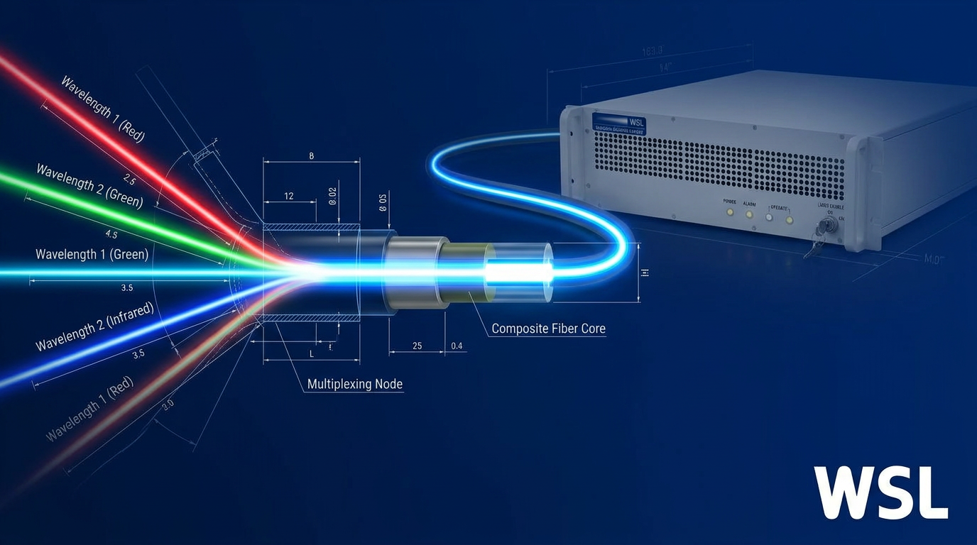
Wavelength division multiplexing is the technology that makes this possible — using different colours of light as independent data lanes, all sharing the same physical fibre simultaneously, without the cost and disruption of laying new cable.
This guide is written for engineers, network professionals, and technical students who want more than a surface-level overview — covering not just the optical physics and CWDM vs DWDM standards, but also active vs passive architectures, vendor lock-in trade-offs, and practical deployment considerations that most treatments leave out.
TL;DR
The physics of wavelength multiplexing is well understood — the harder problem is the engineering. Channel planning, architecture selection, component specification, and vendor strategy each shape whether a WDM network delivers on its capacity promise over the long term. Understanding those decisions, not just the underlying optics, is what separates a network that scales cleanly from one that doesn't.
This article covers:

WDM optical physics: sharing a single fibre
CWDM vs DWDM: channel spacing and ITU standards
Key system components: multiplexers, OADMs, and optical amplifiers
Active vs passive WDM architectures
Technical challenges: crosstalk, dispersion, polarisation effects, and OSNR
Practical deployment, troubleshooting, and vendor lock-in considerations
What is wavelength division multiplexing?
A single strand of glass fibre can carry far more data than any single laser transmitting through it. Wavelength division multiplexing is the technology that closes that gap — by sending dozens of independent light signals down the same fibre simultaneously, each on its own distinct wavelength.
Wavelength division multiplexing (WDM) is a fibre-optic transmission technique that combines multiple optical carrier signals onto a single fibre by assigning each signal its own unique wavelength of light, allowing them all to travel simultaneously without interfering with one another.
The physics that makes this possible is wavelength superposition: different wavelengths of light propagating through a single-mode optical fibre behave independently of each other, much like different colours of light passing through the same pane of glass without mixing.
Picture red, green, and blue light travelling together down the same glass strand. Each colour carries its own stream of data; none of them disrupts the others. WDM scales this principle to tens or hundreds of tightly spaced infrared wavelengths, each acting as a completely separate data path.
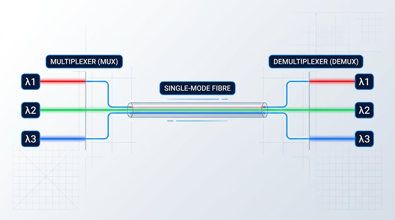
The key abstraction to hold onto throughout this guide is the wavelength-as-channel concept: each wavelength is not just a colour of light, it is a fully independent data channel with its own transmitter, receiver, and data stream.
Where a conventional fibre link is a single-lane road, a WDM system is a multi-lane motorway — each lane invisible to the others, all sharing the same physical infrastructure.
WDM is the optical equivalent of frequency-division multiplexing (FDM) in radio communications: both techniques divide a shared transmission medium into separate frequency (or wavelength) slots, each carrying an independent signal. Engineers familiar with RF systems will recognise the underlying principle immediately.
WDM systems operate within the 1260–1625 nm wavelength range because this is the low-loss transmission window of silica glass fibre — the band where the fibre absorbs and scatters the least light, allowing signals to travel the greatest distances with minimal degradation.
Multiplexer and demultiplexer: the two core components
Every WDM link relies on two essential hardware elements at its ends: a multiplexer at the transmit side and a demultiplexer at the receive side.
- Multiplexer (Mux): Combines multiple individual wavelength signals from separate transmitters onto a single output fibre for onward transmission.
- Demultiplexer (Demux): Separates the combined multi-wavelength signal back into individual wavelengths, routing each to its corresponding receiver.
Critically, the same passive optical device can perform either function depending on the direction of signal flow — which is why the terms mux and demux are often used interchangeably in practice, and why a single unit is frequently deployed at both ends of a bidirectional link.
The practical consequence of this architecture is profound: fibre capacity scales by adding wavelength channels, not by laying new cable. A fibre that carries one channel today can carry tens or hundreds tomorrow, simply by deploying additional transceivers and expanding the mux/demux configuration.
A further advantage is protocol transparency: because each wavelength channel is optically independent, signals running different data formats, protocols, or bit rates can coexist on the same fibre without any awareness of each other.
In a WDM system, wavelengths do not share bandwidth — each one is a discrete, isolated data path. This means capacity grows by adding channels, and different protocols can coexist on the same fibre without modification.
This distinguishes WDM from time-division multiplexing (TDM), where a fibre's capacity is divided into time slots shared among data streams — a scheme that requires all channels to operate at the same bit rate and protocol, imposing rigid uniformity that WDM does not.
WDM itself is not a single standard but a family of technologies, and the most important distinction within that family is between coarse and dense variants — each suited to different distance, density, and cost requirements. That distinction is the subject of the next section.
CWDM vs DWDM: channel spacing, ITU standards, and when to use
Every consequential difference between coarse WDM (CWDM) and dense WDM (DWDM) traces back to a single parameter: channel spacing. That one variable determines what laser technology is viable, how many channels fit on a fibre, how far the signal can travel, and what the system ultimately costs.
CWDM is governed by ITU-T G.694.2, which defines 18 nominal central wavelengths from 1271 nm to 1611 nm with a uniform spacing of 20 nm. The wide spacing is deliberate: it accommodates uncooled DFB lasers, whose output wavelength drifts across a range of roughly ±6–7 nm as temperature changes during operation. Because the channel guard band is wide enough to absorb that drift, CWDM systems need only wideband thin-film filters and thermally uncontrolled laser sources — both of which are significantly cheaper to manufacture and consume less power.
DWDM operates under ITU-T G.694.1, which defines a frequency grid anchored at 193.1 THz supporting fixed channel spacings of 100 GHz, 50 GHz, 25 GHz, and 12.5 GHz. At 100 GHz spacing, adjacent channels are separated by only ~0.8 nm in the C-band — far less than the natural drift of an uncooled laser. DWDM therefore requires temperature-stabilised (cooled) lasers with tight wavelength control, along with precision narrowband filters capable of resolving sub-nanometre channel windows.
The 2020 edition of G.694.1 (Edition 3.0) introduced a flexible DWDM grid, allowing variable channel slot widths defined in 12.5 GHz increments rather than fixed spacings. This accommodates modern coherent modulation formats — such as DP-QPSK and higher-order QAM — where the optimal channel bandwidth depends on baud rate and modulation order rather than a fixed grid. The flexible grid is the mechanism by which DWDM continues to evolve for high-capacity systems; it is very much in active use.
Capacity, reach, and cost: the trade-offs
The table below compares CWDM and the principal DWDM spacings across the dimensions that matter most for system selection.
| Parameter | CWDM | DWDM 100 GHz | DWDM 50 GHz | DWDM 25 GHz / Flex |
|---|---|---|---|---|
| ITU standard | G.694.2 | G.694.1 | G.694.1 | G.694.1 (Ed. 3.0) |
| Channel spacing | 20 nm (~2500 GHz) | 100 GHz (~0.8 nm) | 50 GHz (~0.4 nm) | 25 GHz / variable |
| Max channels per fibre | 18 (C-band use: up to 16) | ~40 | ~80 | ~160+ |
| Typical unamplified reach | Up to ~80 km | Up to ~80 km | Up to ~80 km | Up to ~80 km |
| Amplified reach (EDFA) | Not viable (wavelengths span beyond C-band) | Hundreds to thousands of km | Hundreds to thousands of km | Hundreds to thousands of km |
| Laser type | Uncooled DFB | Cooled (temp-stabilised) DFB | Cooled (temp-stabilised) DFB | Cooled (temp-stabilised) DFB |
| Relative first-in cost | Baseline (lower) | ~30–40% higher than CWDM | Higher than 100 GHz | Highest (coherent DSP required) |
| Primary deployment context | Metro access, enterprise campus, short-haul | Metro core, regional, long-haul | Long-haul, high-capacity terrestrial | Submarine, DCI, ultra-high-capacity |
Side-by-side comparison of CWDM and DWDM variants across channel spacing, maximum channel count, unamplified reach, laser type, relative cost, and typical deployment context.
The pattern in the table is clear: CWDM optimises for cost and simplicity at the expense of scale, while each successive DWDM spacing trades higher component cost and complexity for greater channel density and, critically, access to long-haul amplification. The cost advantage of CWDM is real — trade press estimates from Lightwave Online put first-in system cost at 30–40% lower than equivalent DWDM deployments — but that advantage only holds when the application does not require more than ~18 channels or reach beyond 80 km.
The reach comparison deserves a closer look, because the 80 km unamplified figure is similar for both technologies — the decisive difference is what happens beyond that point. DWDM channels, concentrated in the C-band (1530–1565 nm), can be simultaneously amplified by erbium-doped fibre amplifiers (EDFAs), enabling reach of hundreds to thousands of kilometres in deployed systems. CWDM channels span from 1271 nm to 1611 nm, well outside the EDFA gain window, so they cannot all be amplified by a single EDFA.
Because CWDM wavelengths span from 1271 nm to 1611 nm, they cannot all be amplified by a single EDFA operating in the C-band (1530–1565 nm). Long-haul amplification is therefore fundamentally incompatible with standard CWDM — the limit is rooted in the physics of erbium-fibre gain, not simply in link loss.
Choosing between CWDM and DWDM
CWDM is the natural fit for metro access, enterprise campus, and short-haul applications: environments where channel counts typically run to 4–8 wavelengths, distances stay within 80 km, and capital cost is a primary constraint. The absence of cooled lasers and precision filters keeps both the initial deployment cost and the ongoing power budget low — advantages that compound over time in cost-sensitive edge and access networks.
DWDM is the right choice wherever the application demands high channel counts, long reach, or both: metro core rings, long-haul terrestrial routes, submarine cables, and data centre interconnect links where 40, 80, or more than 160 channels per fibre are needed. At those channel counts and distances, DWDM is not merely preferable — it is the only viable technology, and the higher component cost becomes the cost of meeting the requirement rather than a trade-off against a cheaper alternative.
With the CWDM/DWDM taxonomy and its engineering consequences established, the next section examines the hardware that implements these systems — and why the channel spacing difference drives fundamentally different component choices for multiplexers, filters, and amplifiers.
Key WDM system components: multiplexers, OADMs, and amplifiers
Understanding CWDM and DWDM as standards is one thing — understanding the physical hardware that implements them is another. Three component classes do the heavy lifting in any wavelength division multiplexer system: the mux/demux units that combine and separate wavelengths, the optical add-drop multiplexers that manage traffic at intermediate nodes, and the optical amplifiers that extend reach across long-haul fibre spans.
Multiplexers and demultiplexers
A multiplexer combines multiple wavelength channels onto a single fibre at the transmit end; a demultiplexer separates them back into individual channels at the receive end.
What is worth understanding is that these are not two distinct devices — the same passive optical component performs both functions depending on signal direction, a consequence of optical reciprocity.
Two technologies dominate practical mux/demux design, and the choice between them is largely driven by channel count and system complexity.
- Thin-film filter (TFF): A cascade of individual wavelength-selective filters, each transmitting one channel and reflecting the rest. Insertion loss accumulates with each added stage, making TFFs best suited to the lower channel counts typical of CWDM applications.
- Arrayed waveguide grating (AWG): A planar waveguide circuit that uses wavelength-dependent interference to route all channels simultaneously to separate output ports — compact, passive, and scalable to the high channel counts required by DWDM.
The architectural difference carries direct system consequences. A thin-film filter cascade adds insertion loss at each stage, so the penalty grows with channel count — manageable for the modest channel plans of CWDM, but impractical for the dense channel stacks of DWDM.
An arrayed waveguide grating routes all channels in a single pass through one planar circuit, which is why it has become the dominant technology for high-density DWDM: the loss profile does not worsen as channel count scales.
AWGs do carry one important sensitivity: their channel routing depends on the refractive index of the waveguide material, which shifts with temperature.
Passive athermal AWG designs compensate for this mechanically, but precision DWDM applications — where channel spacing is 50 GHz or 100 GHz and wavelength tolerances are tight — typically use active temperature control to hold the AWG on the ITU grid.
Optical add-drop multiplexers (OADMs)
A pure mux/demux pair at each node would require demultiplexing the entire wavelength stack, processing every channel, and remultiplexing — an expensive and disruptive approach for a node that only needs to access one or two channels out of dozens.
The optical add-drop multiplexer solves this by extracting (dropping) or inserting (adding) specific wavelength channels at an intermediate node while all other channels pass through in the optical domain, untouched.
Fixed OADMs (FOADMs) add and drop a predetermined set of wavelengths defined at installation time, using static filter elements.
They are simple, reliable, and cost-effective — but any change to which wavelengths are added or dropped requires physical intervention: swapping filter modules or rerouting fibre connections.
For stable, predictable traffic patterns where the wavelength plan will not change, FOADMs remain a practical and economical choice.
Reconfigurable OADMs (ROADMs) replace static filters with electronically controlled switching elements — principally wavelength selective switches (WSS) and LCoS (liquid crystal on silicon) spatial light modulators — allowing the add/drop configuration to be changed remotely via software without any physical intervention.
ROADMs were commercially introduced around 2002 alongside DWDM networks, and they define modern flexible optical networking.
The operational flexibility of a ROADM is described across three dimensions, each adding capability at increasing cost and complexity.
- Colorless: Any port can handle any wavelength — there is no fixed binding between a port and a specific channel.
- Directionless: Any wavelength channel can be routed to any fibre direction from the node, without physical reconfiguration.
- Contentionless: The same wavelength can be simultaneously added or dropped on multiple ports without signal contention.
A fully colorless, directionless, and contentionless ROADM offers maximum operational flexibility — but each dimension adds switching hardware, control plane complexity, and cost, so the right level of flexibility is an engineering decision tied to the traffic model of the network.
Erbium-doped fibre amplifiers (EDFAs)
Without optical amplification, fibre attenuation limits a WDM link to roughly 80–100 km before signal quality degrades beyond recovery.
The erbium-doped fibre amplifier overcomes this by amplifying optical signals directly — without converting them to electrical form and back — across the 1530–1625 nm window.
Its decisive system-level advantage is that a single EDFA amplifies every WDM channel simultaneously, making it far more practical than per-channel optical-to-electrical-to-optical (O-E-O) regeneration for multi-channel long-haul links.
EDFAs operate across two gain bands: the C-band (1530–1565 nm) covers the vast majority of long-haul DWDM deployments, while the L-band (1565–1625 nm) extends capacity in high-traffic systems where the C-band is fully loaded.
Because erbium gain is not uniform across the full band, gain-flattening filters are used to equalise signal power across channels — without them, channels at the edges of the gain spectrum arrive with significantly different power levels, degrading system margin.
On the noise side, amplified spontaneous emission (ASE) is the principal impairment: erbium ions emit photons spontaneously as well as in response to the signal, adding broadband noise to every amplified channel.
Practical EDFAs carry a noise figure in the range of 4–6 dB, and in a long-haul link with many cascaded amplifier stages, each stage contributes ASE — making OSNR management the central system design constraint over tens of spans.
DWDM channel plans are deliberately designed to sit within the EDFA C-band window (1530–1565 nm). CWDM wavelengths span well outside this range, which is why CWDM links cannot be amplified by standard EDFAs and are therefore reach-limited to a single fibre span.
For DWDM systems, EDFA selection is not a commodity decision — operating band, channel count, span loss, and power budget all interact, and an amplifier specified to the actual operating conditions of the deployment will outperform a fixed-catalogue module in any demanding application.
Woodrow Scientific Limited's Custom EDFA is built on exactly this principle: engineered end-to-end to the application rather than drawn from a fixed specification sheet, with every parameter — operating band (C-band, L-band, or dual C+L), output power, pulse regime, cooling, form factor, and control firmware — configured to the deployment.
WSL is a UK manufacturer founded in 2012 that designs, builds, qualifies, and supports its amplifiers entirely in-house on patented technology, with engineering expertise rooted in Southampton's Optoelectronics Research Centre — the institution where the EDFA was originally developed.
This matters in practice: many suppliers in the EDFA market are resellers or importers of fixed-spec modules, without the in-house engineering capability to adapt a design, accelerate a fix, or support a demanding integration.
The platform scales to the leading commercially available power levels for erbium fibre — pulse energies above 10 mJ, peak powers above 100 kW, and average powers above 100 W — making it a credible choice for the most demanding long-haul and high-power applications.
With the three principal WDM component classes established, the next question is how they are combined at the system level — specifically, which components are present in a passive architecture versus an active one, and what that distinction means for network design and reach.
Active vs passive WDM architectures
Most WDM reference material treats the CWDM vs DWDM choice as the central architectural decision and stops there. It isn't. The more consequential question — one that shapes power infrastructure, operational staffing, management complexity, and upgrade costs for a decade or more — is whether the system is built around passive optical components or incorporates active elements in the optical path.
A passive WDM system is composed entirely of components that require no electrical power to function: multiplexers, demultiplexers, and fixed OADMs. Signal routing is determined by the optical filtering built into those components at the time of installation, and nothing in the optical path consumes power or requires management infrastructure.
An active WDM system introduces powered elements into that path — EDFAs for amplification, ROADMs for electronically controlled wavelength routing, and transponders for signal regeneration and format conversion. Each of those elements requires power, generates heat, and demands ongoing operational support.
Passive WDM: strengths and hard limits
The practical advantages of passive architectures are substantial. There is no power infrastructure to provision at intermediate field sites, no active equipment to fail between maintenance windows, and commissioning is straightforward once the optical budget is verified.
Passive CWDM systems dominate metro access, enterprise campus, and short-haul applications precisely because, in those contexts, passive is not the budget compromise — it is the correct engineering answer.
The limitations are equally clear. Reach is bounded by the available optical power budget: without amplification, unamplified passive systems are typically constrained to spans under 80 km, and real-world budgets often impose tighter limits depending on channel count and fibre loss.
Channel count is fixed at deployment. Adding a wavelength to a passive system means physical intervention — swapping or adding mux/demux hardware — which typically requires a maintenance window and a site visit. There is no remote reconfigurability, and management visibility is limited to endpoint monitoring: no intermediate node can report on signal quality or be used to equalise power across channels.
Active WDM: capability and operational cost
Active architectures remove the reach and scalability constraints that bound passive systems. EDFA amplification extends spans to hundreds of kilometres on terrestrial networks and thousands on submarine systems. ROADMs allow wavelengths to be added, dropped, or rerouted from a network management console without a truck roll — a capability that becomes operationally essential as traffic patterns shift.
Intermediate nodes in an active network can monitor optical signal-to-noise ratio, equalise channel power, and isolate faults to a specific span — capabilities that are simply absent in passive architectures.
The operational cost reality is frequently underweighted in first-cost comparisons. Every active element at an intermediate site requires mains power or generator backup, environmental controls to manage heat dissipation, maintenance contracts, and operations staff with the skills to manage the equipment.
These ongoing operational expenditures — power, cooling, maintenance, and staffing — can dwarf the initial capital cost difference between a passive and active deployment over a five- to ten-year asset life. An operator who prices the capex but not the opex is not doing a complete comparison.
It is also worth noting that active systems, with their managed transponders and ROADM control planes, introduce vendor and management dependencies that passive systems do not — a dimension covered in more depth later in this guide.
Matching architecture to deployment context
The table below maps the two architectures against the deployment parameters that drive the decision: distance, channel count, reconfigurability requirements, and typical application contexts.
| Parameter | Passive WDM | Active WDM |
|---|---|---|
| Typical max reach (unamplified) | Up to ~80 km, often less depending on fibre loss and channel count | Hundreds to thousands of km with EDFA amplification |
| Channel count | 4–40 channels, fixed at installation | 40–160+ channels, dynamically configurable with ROADMs |
| Reconfigurability | None — physical intervention required to change routing | Remote, software-driven via ROADM control plane |
| Intermediate site power | Not required — no powered elements in optical path | Required at each amplifier/ROADM site (mains or generator) |
| Management visibility | Endpoint monitoring only | Per-node OSNR, power, and fault monitoring |
| Typical applications | Enterprise campus, metro access, CATV distribution, short-haul DCI | Long-haul terrestrial, submarine, metro core rings, large-scale DCI |
| Operational complexity | Low — passive components have no failure modes requiring active management | High — requires trained NOC staff, maintenance contracts, cooling systems |
Side-by-side comparison of passive and active WDM architectures across key deployment parameters to support architectural decision-making.
The table makes the trade-off structure visible: passive systems win on simplicity, cost of ownership at short distances, and operational burden; active systems win on reach, scale, and flexibility. The crossover point is not a fixed distance or channel count — it depends on the operator's traffic growth projections, staffing model, and tolerance for operational complexity.
A short-haul metro access ring with stable, predictable traffic and no requirement for dynamic rerouting is a passive deployment. A metro core ring carrying aggregated traffic from dozens of access nodes, where any wavelength may need to be rerouted within hours of a topology change, is an active one.
Operators who choose passive architectures primarily to minimise upfront cost — without modelling traffic growth — risk a forced upgrade to active infrastructure within a few years. At that point, the passive capex is sunk and the active infrastructure must be added on top. The cost of the wrong first decision compounds. Architecture should be selected for the network's expected state in year five or ten, not year one.
The converse trap is equally real: deploying active infrastructure where passive would suffice for the foreseeable operating life adds unnecessary power draw, cooling requirements, and management burden without delivering any operational benefit.
The right architectural question is not "which is cheaper to buy?" but rather: what distance must the system cover, how many channels are needed now and in three years, does the operator have the staffing to manage active nodes, and what does the traffic growth forecast look like? Those inputs determine the architecture — not the line-item price of the hardware.
With the architectural framework established, the next layer of understanding is what can go wrong within whichever system is deployed: the optical impairments and engineering challenges that practitioners must account for regardless of whether the network is passive or active.
Technical challenges in WDM systems
Every impairment that degrades a WDM system was predictable at design time — the engineers who treat these phenomena as operational surprises are the ones who face expensive mid-life remediation.
The physics of multi-wavelength propagation through fibre introduces a set of distinct impairment classes, each with its own origin, severity conditions, and mitigation strategy.
Crosstalk: linear and nonlinear mechanisms
Crosstalk — the leakage of power from one channel into another — arises through two fundamentally different mechanisms that require different solutions.
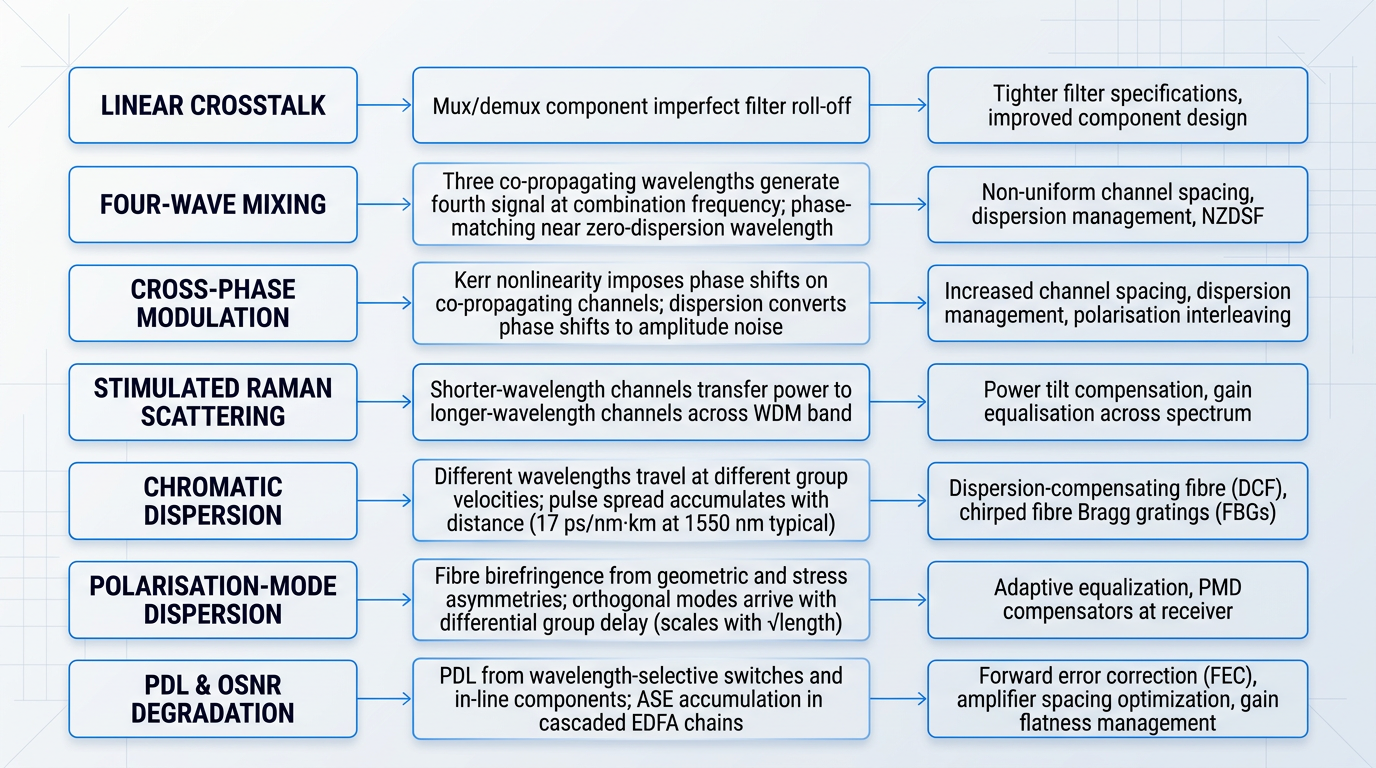
Linear crosstalk originates in the mux/demux components themselves: imperfect filter roll-off allows adjacent channel power to bleed through the passband of a neighbouring channel, and the remedy lies in tighter filter specifications and improved component design.
Nonlinear crosstalk is a fibre-physics problem, not a component problem — it arises when high launch powers drive the fibre into nonlinear operating regimes, and it cannot be resolved by improving filter quality.
Three distinct nonlinear mechanisms matter to WDM system designers, each with different severity conditions and mitigations.
Four-wave mixing (FWM)
Three co-propagating wavelengths interact to generate a fourth signal at a combination frequency that can land directly on an occupied channel.
Four-wave mixing is most severe on equally-spaced channel grids near the fibre's zero-dispersion wavelength, where phase-matching conditions allow the interaction to build coherently over long distances.
Mitigations include non-uniform channel spacing, dispersion management, and the use of non-zero dispersion-shifted fibre (NZDSF), all of which disrupt the phase-matching conditions that allow FWM to accumulate.
Cross-phase modulation (XPM)
Intensity fluctuations in one channel impose phase shifts on co-propagating channels through the Kerr nonlinearity; chromatic dispersion then converts those phase shifts into amplitude noise at the receiver.
Cross-phase modulation is most severe for narrowly spaced DWDM channels, where walk-off between channels is slow and the interaction accumulates over longer fibre lengths.
Available mitigations include increased channel spacing, dispersion management to accelerate walk-off, and polarisation interleaving of adjacent channels.
Stimulated Raman scattering (SRS)
Stimulated Raman scattering causes shorter-wavelength channels to act as optical pumps, transferring power into longer-wavelength channels across the WDM band.
The primary consequence is a power tilt across the channel spectrum — a gain-equalisation concern in wide-band systems rather than a per-channel crosstalk problem in the strict sense.
Chromatic dispersion
Chromatic dispersion arises because different wavelengths travel at slightly different group velocities in fibre, causing transmitted pulses to spread as they propagate — an effect that accumulates with distance and becomes more damaging as data rates increase.
Standard single-mode fibre (SMF) exhibits a dispersion coefficient of approximately 17 ps/(nm·km) at 1550 nm as a widely cited typical value, meaning a pulse carried on a channel 1 nm wide accumulates roughly 17 picoseconds of spread per kilometre of fibre.
The two principal compensation techniques are dispersion-compensating fibre (DCF), inserted in-line to provide negative dispersion that partially cancels accumulated SMF dispersion, and chirped fibre Bragg gratings (FBGs), which reflect different wavelengths at different depths to achieve a compact, low-loss compensating delay.
Zero-dispersion fibre is incompatible with multi-channel WDM: near-zero dispersion conditions maximise four-wave mixing and cross-phase modulation, making it the worst possible medium for dense channel grids. The design challenge is not to eliminate dispersion but to maintain controlled, non-zero dispersion across all channels — enough to suppress nonlinear interactions, not so much that pulse spreading limits reach.
Non-zero dispersion-shifted fibre (NZDSF) was developed precisely to navigate this trade-off, providing enough residual dispersion to suppress FWM while keeping accumulated dispersion manageable over long spans.
Polarisation effects: PMD and PDL
Polarisation introduces two distinct impairment mechanisms that are frequently conflated but have entirely different physical origins: polarisation-mode dispersion (PMD) is a fibre-physics effect, while polarisation-dependent loss (PDL) is a component effect.
Polarisation-mode dispersion
Real fibre is not perfectly circular — slight geometric and stress asymmetries produce birefringence, causing the two orthogonal polarisation modes of each channel to travel at marginally different velocities and arrive at the receiver with a differential group delay that broadens the pulse.
PMD is stochastic in character: the differential group delay varies unpredictably with temperature and mechanical stress, making it impossible to compensate with a fixed optical element in the way that chromatic dispersion can be addressed.
PMD scales with the square root of fibre length, and it becomes a dominant impairment at higher line rates — typically cited as a threshold around 10 Gbps and above — making it a particular concern when upgrading legacy fibre plant to higher-speed WDM operation.
Polarisation-dependent loss
PDL is differential attenuation of signal power as a function of polarisation state, arising primarily from wavelength selective switches and other in-line optical components rather than from the transmission fibre itself.
In cascaded optical paths, PDL accumulates and degrades the optical signal-to-noise ratio (OSNR), with the effect most pronounced in coherent systems where polarisation state is tracked and exploited for capacity.
OSNR degradation in cascaded amplifier chains
In long-haul WDM systems, OSNR management is the central design challenge — not one consideration among several, but the fundamental constraint that determines how far a signal can travel before regeneration becomes necessary.
Each EDFA stage adds amplified spontaneous emission (ASE) noise across the amplified band, and this noise accumulates with every successive span: a system traversing tens of amplifier stages carries a corresponding accumulation of ASE, all of which competes with signal power at the receiver.
Amplifier spacing, gain flatness across the WDM band, and forward error correction (FEC) are the primary design levers for managing accumulated OSNR — FEC in particular allows the system to operate closer to the noise floor by tolerating a higher raw bit error rate before correction.
The diagram below maps each major WDM impairment to its physical origin and primary mitigation, providing a consolidated reference for the categories covered in this section.
Wavelength stability requirements
DWDM systems operating on 50 or 100 GHz channel grids require laser centre frequencies to be held within a very tight tolerance of their assigned ITU grid frequency — typically cited as approximately ±1–2 GHz as a representative industry figure — a precision engineering requirement that immediately distinguishes DWDM transmitter design from CWDM, where uncooled lasers with much wider frequency tolerances are acceptable.
Temperature-stabilised lasers and active wavelength locking — using feedback from an on-board wavelength reference to continuously correct the laser drive current or temperature setpoint — are standard practice in DWDM transceivers precisely because passive thermal drift cannot meet this tolerance.
Wavelength drift beyond the channel guard band is among the most common fault signatures encountered in deployed DWDM systems, and recognising it is a foundational skill in the commissioning and troubleshooting discipline covered in the next section.
Need an EDFA Tailored to Your WDM System?
Dispersion, OSNR degradation, and wavelength stability challenges all demand the right amplification. Woodrow Scientific builds custom EDFAs for a wide range of optical communications applications.

Practical deployment and troubleshooting considerations
Understanding WDM in theory and deploying it successfully are two different disciplines. The impairments covered in the previous section — chromatic dispersion, PMD, OSNR degradation, wavelength stability — do not announce themselves at commissioning; they surface later, in degraded performance, unexplained outages, and expensive remediation. The engineers who avoid those outcomes are the ones who treat deployment as a structured engineering process, where every decision made at design time is deliberately connected to an operational outcome.
Fibre plant requirements
Before any WDM equipment is selected, the fibre plant itself must be characterised — because the fibre is not a neutral medium, and its physical properties directly constrain what the system can do.
The two most relevant standards are G.652 (standard single-mode fibre, by far the most widely deployed) and G.655 (non-zero dispersion-shifted fibre, NZDSF), which differ primarily in their dispersion characteristics across the C- and L-bands.
G.655 NZDSF was designed to reduce the four-wave mixing impairments that arise when dispersion is too close to zero, while still keeping dispersion low enough to limit chromatic spreading — a balance that affects amplifier spacing decisions in long-haul DWDM design.
The PMD constraints discussed earlier become a hard practical limit when legacy fibre is involved: older installed plant with high PMD coefficients can restrict upgrade paths to 10 Gbps and above, where polarisation-mode dispersion becomes system-limiting rather than merely a budgeted impairment.
The practical implication is that fibre characterisation — measuring actual PMD, attenuation, and chromatic dispersion across the planned wavelength range — must precede equipment selection, not follow it.
Optical power budgeting
A link budget is the accounting of all optical power gain and loss between transmitter and receiver, and it is the foundational design document for any WDM span.
The budget must account for transmitter output power, insertion loss at each multiplexer, demultiplexer, and OADM, fibre attenuation across the span, connector and splice losses, and the minimum receiver sensitivity required for the target bit error rate.
A minimum power margin of approximately 3 dB is standard engineering practice — this headroom protects against connector degradation over time, component ageing, and the measurement uncertainty inherent in any real installation.
Critically, the budget must be calculated per channel across the full wavelength range, not as a single aggregate figure. Insertion loss in WDM components is not spectrally flat: a channel at the edge of the passband can carry significantly more loss than one at the centre, and a budget that passes at the design wavelength may fail at the band edge.
This per-channel loss variation is precisely why channel power equalisation — through gain-flattening filters and variable optical attenuators (VOAs) — is a design requirement rather than an optional refinement.
Amplifier span planning
In amplified DWDM systems, EDFA placement is driven by span loss, not by distance — the target is typically 20–25 dB of span loss per amplifier stage, and amplifiers are positioned to meet that target across the route.
Equal span loss intervals are the goal because unequal spans create an uneven OSNR accumulation profile: channels traversing a longer, higher-loss span arrive at their amplifier with degraded OSNR, while channels on a shorter span may be over-amplified, increasing nonlinear impairments.
OADM nodes introduce a specific power management challenge: a channel added at an OADM enters the system at a different power level than the pass-through channels it joins, and without correction this imbalance propagates and compounds through subsequent amplifier stages.
The standard solution is a booster amplifier placed immediately after the OADM, combined with VOAs on the added channels to equalise their power relative to pass-through traffic before the signal enters the next span.
System commissioning procedure
Commissioning is the moment when design-time assumptions are verified against physical reality — and it is the source of the baseline data that makes all future troubleshooting possible.
The correct order of operations begins with the fibre plant, before any WDM equipment is connected. An OTDR sweep of each span establishes baseline attenuation, locates high-loss splices, identifies reflections, and confirms fibre continuity — catching plant problems before expensive equipment enters the signal path.
All optical connectors should be inspected and cleaned before connection; contaminated connectors are the most common source of unexplained insertion loss, and cleaning at commissioning prevents avoidable measurement errors from entering the baseline record.
- Characterise the fibre plant: OTDR sweep of every span: measure attenuation, locate splices, confirm continuity. Inspect and clean all connectors before connection.
- Verify span loss per channel: Confirm that measured span loss falls within the design budget for each channel across the full wavelength range.
- Bring up channels and measure with OSA: Use an optical spectrum analyser to confirm channel wavelengths, per-channel power levels, and OSNR for every populated channel.
- Document all baseline measurements: Record OSA readings, OTDR traces, and power levels as the commissioning baseline — the reference for all future performance comparisons.
- Verify amplifier gain and VOA settings: Confirm EDFA gain and VOA attenuation values match design targets; adjust for any channel power imbalance identified in the OSA sweep.
The baseline OSA measurements documented at commissioning are not administrative overhead. Without them, it is impossible to distinguish between a channel that was always marginally weaker and one that has genuinely degraded — a distinction that determines whether a fault requires investigation or is within normal operating tolerance.
Troubleshooting methodology
Effective fault isolation in a WDM system depends on a structured mental model, not a checklist. The first question to answer is always: how many channels are affected?
Faults affecting all channels simultaneously point to a shared element — an amplifier, a fibre span, or a common connector. Faults affecting only one or two channels point to a channel-specific element — a transmitter, a per-channel filter, or a connector on that path alone. This distinction alone cuts the fault search space dramatically before a single measurement is taken.
Once the scope is established, OSA measurements at intermediate points along the link localise the fault to a specific span or node. The most efficient isolation direction is from receiver back toward transmitter: the receiver is where the problem is observed, and working upstream identifies the last point at which the signal was within specification.
The principal fault types and their first-line checks are consistent across most DWDM deployments:
- Channel power imbalance: Check amplifier gain settings and VOA values first, then inspect connector cleanliness on the affected channel before assuming component failure.
- Wavelength drift: Check transmitter temperature control and laser bias current. In DWDM systems, wavelength drift is almost always a thermal or bias issue, not a hardware failure.
- OSNR degradation: Check span loss and amplifier noise figure. Elevated span loss forces higher amplifier gain, increasing ASE noise and degrading OSNR across all channels on that span.
- Connector degradation: Clean and inspect all optical connections before replacing any component. Contaminated connectors are the most common cause of unexplained power loss in deployed systems.
The connector cleanliness point warrants emphasis: it recurs as the root cause in a disproportionate share of field faults, yet it is consistently the last thing checked rather than the first.
Test equipment essentials
Four instrument types cover the full scope of WDM deployment and maintenance work; each has a distinct and non-substitutable role.
- OTDR: Fibre characterisation, span loss measurement, and fault location. The essential tool for pre-commissioning fibre plant verification and post-fault span diagnosis.
- Optical spectrum analyser (OSA): Measures channel wavelengths, per-channel power levels, and OSNR simultaneously. The primary diagnostic instrument for any WDM system.
- Optical power meter: Span loss verification and rapid power-level checks. Faster than an OSA for quick pass/fail checks where spectral detail is not required.
- CD and PMD analysers: Chromatic dispersion and polarisation-mode dispersion measurement. Required for high-speed links at 10 Gbps and above, where these impairments become system-limiting.
For short-reach or passive CWDM deployments, the OTDR and optical power meter typically suffice; the OSA and dispersion analysers become indispensable as channel count, bit rate, and span length increase.
Having covered the engineering disciplines that govern how a WDM system is built and maintained, the next consideration shifts from operational practice to a strategic dimension that shapes what system you can deploy in the first place: the trade-offs between proprietary WDM architectures and open, interoperable alternatives.
Vendor lock-in and open WDM architectures
The vendor choice an operator makes when deploying a WDM system rarely constrains them for just a few years — it typically shapes their procurement options, upgrade cycles, and operational costs for a decade or more.
Traditional WDM systems were architected as closed, single-vendor stacks: line systems, transponders, amplifiers, and management software were tightly integrated, with proprietary interfaces between every functional layer that made mixing equipment from different vendors practically impossible.
This is not purely a historical condition — a significant portion of deployed infrastructure still operates this way, and understanding where the lock-in actually lives in the system is the first step to evaluating it.
- Proprietary channel plans: Vendor-specific wavelength grids that deviate from ITU standards prevent third-party transponders from operating on the same line system.
- Vendor-specific FEC algorithms: Proprietary forward error correction implementations require matched transponders at both ends of a link — interoperability demands open or shared FEC instead.
- Closed NMS/EMS interfaces: Management systems with no standard APIs force operators to use the incumbent vendor's software tools, limiting automation and integration options.
- Proprietary gain management: Vendor-specific OSNR control and amplifier gain algorithms tie optical performance optimisation to a single vendor's end-to-end implementation.
The operational consequences of these mechanisms compound over time: operators cannot source replacement transponders from alternative vendors, upgrade cycles follow the incumbent vendor's product roadmap rather than the operator's traffic growth, and the total cost of ownership often exceeds what the initial capital cost implied — because the operator has no competitive leverage at renewal.
This structural asymmetry between vendor and operator is what motivated the industry's collaborative response: the OpenROADM MSA.
OpenROADM MSA and network disaggregation
Founded in 2015 by a group of network operators and equipment vendors, the OpenROADM MSA is a community that defines and promotes carrier-focused open API models and optical specifications, with the explicit goal of reducing vendor lock-in and giving operators greater flexibility, choice, and control over their optical networks.
The MSA's approach is built on a disaggregated architecture: separating network functions and equipment into smaller, independently sourceable components — line system, transponders, pluggable optics, and control plane — so that operators can choose the best components from multiple vendors without being locked into a single vendor's solution.
One of the most commercially significant concepts this enables is the alien wavelength: a third-party transponder transported over an incumbent vendor's line system infrastructure, decoupling transponder procurement from line system procurement entirely.
This decoupling matters because transponders represent a substantial share of total DWDM system cost — industry sources cite figures ranging from 60% to over 70% of full system costs — making multi-vendor deployment of transponders a lever with real commercial weight, not just architectural elegance.
The OpenROADM MSA acknowledges directly that interoperability requires the use of open or shared forward error correction (FEC), Probabilistic Constellation Shaping (PCS), and optical power control algorithms, rather than the proprietary implementations that are highly optimized in single-vendor systems. Open ROADM optical specifications are considered a baseline — meaning a fully optimised closed system on the same physical infrastructure may outperform an open multi-vendor deployment on a per-link basis.
This trade-off is not a minor footnote: certain design and operational techniques that rely on optimised end-to-end control or real-time communications between components may simply not be feasible when different vendors' implementations sit at both ends of a link.
Operators evaluating open architectures need to weigh this performance baseline against the strategic benefits of disaggregation — the right answer depends on the specific fibre plant, reach requirements, and the operator's tolerance for integration complexity.
Who benefits from open architectures?
Large operators with substantial in-house optical engineering capability — teams able to manage multi-vendor integration, maintain their own NMS integrations, and evaluate component performance independently — are best positioned to capture the benefits of open architectures.
Smaller operators may find that a single-vendor integrated system is simpler to deploy and lower-risk to operate, even if it carries long-term strategic constraints; the integration overhead of a disaggregated network is itself a real operational cost that should be counted honestly.
The open-versus-closed choice is not a universal recommendation — it is a fit-for-purpose engineering decision that should be grounded in the operator's scale, growth trajectory, and internal capability, not in vendor advocacy or incumbent inertia.
One further dimension deserves attention at the component level: for demanding WDM applications — high-power amplification, specialised operating bands, long-haul DWDM — the distinction between a genuine manufacturer and a reseller or importer matters beyond procurement.
A manufacturer with in-house design, build, and support capability can provide engineering assistance during integration, supply spares from its own production line, and make product improvements over the system lifetime; a reseller cannot do these things because it does not own the engineering.
With the vendor and architecture landscape now mapped alongside the technical and operational foundations covered earlier, the next step is to see where WDM is actually deployed — from long-haul terrestrial networks and submarine cables through to metro, data centre interconnect, and emerging quantum communications applications.
WDM Applications: From Long-Haul to Quantum
Every technical concept covered in this guide — channel spacing, EDFA amplification, OSNR budgets, ROADM reconfigurability, coherent modulation — exists because specific real-world applications demanded it. Surveying where wavelength division multiplexing is actually deployed shows not just where the technology is used, but why each domain pushed its development in a particular direction.
Long-Haul Terrestrial Networks
Long-haul terrestrial infrastructure is the domain most closely associated with DWDM, and for good reason: it is where the technology first proved itself at commercial scale, with early deployments beginning in the mid-1990s.
The capacity story is one of sustained compounding growth. Early DWDM systems carried a handful of channels at 2.5 Gbps each; today, a single fibre pair can deliver multi-terabit aggregate throughput by combining high channel counts with per-channel rates of 100 Gbps, 400 Gbps, and beyond.
This scaling has been made possible by the C-band EDFA amplification chain discussed in the components section — cascaded amplifiers spaced at regular intervals regenerate the entire WDM comb simultaneously, making distance largely an engineering parameter rather than a physical barrier.
Long-haul terrestrial networks also drove the development of coherent detection and advanced modulation formats, as operators pushed for more bits per hertz of spectrum across existing fibre plant rather than deploying new cable.
Submarine Cable Systems
Submarine cable systems represent the most demanding DWDM deployment environment. Modern systems deliver over 200 Tbps of lit capacity across tens of thousands of kilometres — carrying the majority of international internet traffic between continents.
Repeaters are placed roughly every 80–100 km along the cable route, each housing EDFA stages that restore signal power across the full WDM channel plan without any electrical regeneration.
What makes submarine systems uniquely demanding is the absence of mid-route intervention. Once a cable is laid, the in-line components are inaccessible for the system's operational lifetime — typically 25 years — so OSNR management must be engineered conservatively from the outset, with no margin for remediation.
The frontier of per-channel capacity on these routes continues to advance. In February 2024, Cisco and Microsoft demonstrated 800 Gbps transmission on the Amitié transatlantic cable — a 6,234 km route from Boston to Bordeaux — using DWDM with 150 GHz channel spacing, achieving a spectral efficiency of 5.33 bit/s/Hz.
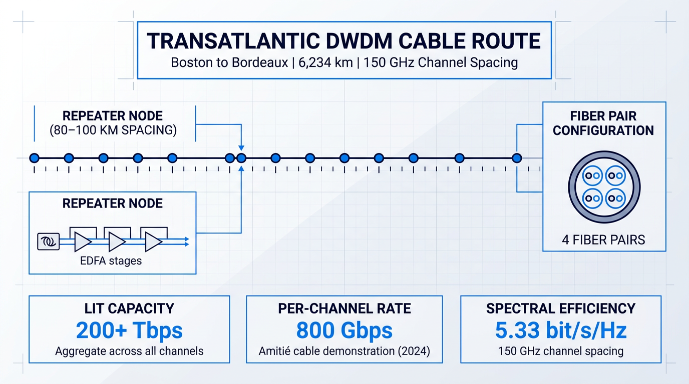
Careful submarine channel planning — allocating wavelengths to maximise capacity while respecting the power and OSNR constraints of the specific cable design — is therefore a critical engineering discipline before a single byte of traffic is lit.
Metro Networks
Metro networks are the domain where the CWDM/DWDM choice is a live engineering and economic decision rather than a foregone conclusion.
At the metro access and edge layer, passive CWDM is well suited: distances are short, channel counts are low, no amplification is required, and the wider 20 nm channel spacing allows the use of uncooled, lower-cost lasers.
In the metro core, the calculus shifts toward DWDM. Longer ring distances, higher traffic densities, and the need for dynamic wavelength management via ROADM-equipped nodes favour the tighter channel spacing and active architecture that DWDM provides.
This layered approach — passive CWDM at the edge feeding into active DWDM at the core — reflects the active versus passive architecture trade-offs covered earlier in the guide, and is the dominant deployment pattern in metropolitan fibre networks today.
Data Centre Interconnect
Data centre interconnect (DCI) has become the most significant growth application for DWDM in the current decade, driven by the bandwidth demands of hyperscale cloud platforms and AI infrastructure.
The key development enabling DCI at scale is the coherent pluggable optics form factor. The OIF 400ZR standard specifies 400 Gbps per wavelength over DWDM links, implemented in compact QSFP-DD modules that plug directly into router and switch ports.
The OpenZR+ MSA extends this to configurable capacities from 100 Gbps to 400 Gbps per wavelength, supporting longer reaches beyond the 120 km ceiling of the base 400ZR specification.
Both standards eliminate the need for separate transponder shelves — the traditional DWDM transport layer — reducing both the physical footprint and cost per bit for operators connecting distributed data centres across metro and regional distances.
By embedding coherent DWDM transmission into a QSFP-DD router port, 400ZR merges the IP and optical transport layers — a structural simplification that changes how DCI networks are designed and operated, not just how they are equipped.
Quantum Communications and Distributed Fibre Sensing
WDM fibre infrastructure is increasingly being extended into two emerging domains: quantum key distribution (QKD) and distributed fibre sensing. Both are genuinely deployed at smaller scale today, with active research and standardisation work ongoing.
The central challenge for QKD coexistence on shared WDM fibre is Raman scattering noise: high-power classical channels generate broadband photon noise that can overwhelm the single-photon-level quantum channels. Research published in Nature confirms that careful wavelength assignment — placing QKD channels in the O-band or at the short-wavelength edge of the C-band, away from the classical traffic band — is the primary mitigation strategy.
Distributed acoustic sensing (DAS) applications similarly leverage the 1550 nm window — the same spectral region that dominates DWDM — because of its low fibre attenuation and compatibility with EDFA amplification. DAS interrogators emit continuous 1550 nm signals and analyse Rayleigh backscatter to detect acoustic and vibrational events along the cable, enabling applications from seismic monitoring to infrastructure sensing.
The breadth of WDM's application landscape — from the 1990s long-haul backbone to transoceanic cable trials and quantum channel coexistence experiments — reflects a technology that has matured through decades of engineering refinement; the Conclusion draws together the key themes that have made that maturity possible.
See WDM Amplification Technology in Real Applications
Woodrow Scientific builds custom EDFAs and free-space optical communications systems for demanding real-world deployments. Explore how their laser comms technology puts WDM principles into practice.
Conclusion
WDM: the technology that scales optical fibre capacity
Wavelength division multiplexing is a mature technology — the physics is settled, the standards are established, and the components are well characterised. What varies between networks that perform and networks that struggle is the quality of the decisions made around that physics.
Ground those decisions in your actual operating requirements: the distances you need to span, the channel counts your traffic demands, and the operational model your team can sustain. The technology will hold up its end.
Frequently asked questions about wavelength division multiplexing
Answers to common questions about WDM technology, CWDM and DWDM standards, system components, and optical signal challenges.
A wavelength division multiplexer is a passive optical device that combines multiple optical signals of different wavelengths onto a single fibre. At the receive end, the same type of device operates as a demultiplexer, separating the combined signal back into individual wavelength channels. Notably, the same physical component can perform both functions: the direction of signal travel determines whether it acts as a multiplexer or demultiplexer. This bidirectional capability distinguishes it from active network components that require separate transmit and receive hardware.
Wavelength division multiplexing works by treating each colour of light as a separate data lane. Just as a motorway carries multiple vehicles in parallel lanes without interference, a single fibre carries many independent data streams simultaneously — each riding a distinct wavelength. The streams share the same physical cable but never mix, giving operators a way to multiply fibre capacity without laying additional cable.
The fundamental difference is channel spacing. CWDM uses 20 nm spacing between channels, supporting up to 18 channels across the O- to L-band. Its wide spacing allows uncooled, lower-cost lasers, but because CWDM wavelengths span beyond the erbium-doped fibre amplifier (EDFA) gain band, amplification is not practical — limiting reach to roughly 80 km per unamplified span. DWDM uses 100 GHz spacing (approximately 0.8 nm) or tighter, fitting 40 to 160 or more channels onto a single fibre. Its narrow spacing requires temperature-stabilised, cooled lasers and is fully compatible with EDFA amplification, enabling reach across hundreds to thousands of kilometres. The right choice depends on three variables: required distance, channel count, and budget. CWDM suits shorter metro and enterprise links where cost is the priority; DWDM is the standard for long-haul, submarine, and high-capacity metro core applications.
Yes — DWDM is the dominant technology for long-haul terrestrial and submarine networks, metro core infrastructure, and high-capacity data centre interconnect. It is not a legacy technology. Modern coherent DWDM systems carry 400 Gbps or more per channel, and aggregate capacities exceeding 10 Tbit/s per fibre pair are deployed in live production networks. Far from being superseded by newer optical approaches, DWDM underpins those approaches: coherent modulation, flexible-grid ROADMs, and advanced forward error correction all operate within the DWDM framework.
Yes. DWDM channels can be positioned within CWDM channel slots, allowing both technologies to operate simultaneously on the same fibre. This coexistence is standards-defined: the ITU-T G.694.1 (DWDM) and G.694.2 (CWDM) channel maps are designed to be compatible. Because each CWDM channel window is 20 nm wide and DWDM channels are spaced at 100 GHz (roughly 0.8 nm), multiple DWDM channels fit comfortably within a single CWDM slot. This makes hybrid deployment a practical upgrade path — operators can add DWDM capacity to an existing CWDM infrastructure without laying new fibre.
An EDFA (erbium-doped fibre amplifier) amplifies all WDM channels simultaneously in the optical domain, without converting signals to electrical form. This all-optical amplification compensates for fibre attenuation over long spans and is the enabling technology for long-haul DWDM: without it, reach would be limited to roughly 80 km per unamplified segment. EDFAs operate primarily in the C-band (1530–1565 nm), which covers the majority of long-haul DWDM deployments. The L-band (1565–1625 nm) is used in high-traffic systems where C-band capacity is exhausted and additional spectral range is needed. Because a single EDFA boosts all channels at once regardless of data rate or modulation format, it scales efficiently as channel counts increase.
Crosstalk in WDM systems falls into two distinct classes. Linear crosstalk arises from imperfect spectral isolation in multiplexer and demultiplexer filters: a filter that does not completely reject adjacent channels allows a fraction of their optical power to leak into the target channel, degrading the signal-to-noise ratio. Nonlinear crosstalk occurs at high launch powers, where fibre nonlinearities generate interference between channels through mechanisms including four-wave mixing (FWM), cross-phase modulation (XPM), and stimulated Raman scattering (SRS). Mitigation relies on a combination of careful channel spacing to reduce nonlinear interaction, dispersion management to suppress FWM phase-matching, and controlled launch power to keep nonlinear effects below threshold. Filter quality in the mux/demux units is the primary lever against linear crosstalk.