

Introduction
If you work with machines that need to move precisely — positioning a tool, synchronising axes, controlling torque under load — you already know that motion control is less a single technology than an engineering discipline.
This guide is written for engineers, automation professionals, and technical buyers who want to understand how that discipline actually fits together: not just the names of the parts, but why each one exists and what happens when they interact.
The goal is a system-level picture — the kind of understanding that makes specifying, integrating, and troubleshooting motion systems considerably less painful.
TL;DR
Motion control rewards engineers who think in systems, not components. The gap between a system that performs reliably and one that frustrates at every integration step almost always comes down to understanding how controllers, drives, motors, and feedback devices work together — not in isolation.
This article covers:

Open-loop vs. closed-loop control architectures
Controllers, drives, and motor types
Actuators, mechanical transmission, and feedback devices
Performance parameters and system integration
Industrial applications across robotics, CNC, and aerospace
AI, IIoT, and Industry 4.0 trends
What is motion control?
Every time a CNC machine cuts a component to tolerance, a pharmaceutical filling line dispenses an exact dose, or a robotic arm welds at a precise coordinate, the same engineering discipline is at work: motion control.
This guide covers motion control as an engineering discipline in industrial automation — distinct from the unrelated use of the term in AI video animation and filmmaking software.
In engineering terms, motion control is the discipline of precisely regulating the position, velocity, torque, and force of machine components — using a coordinated system of hardware and software — to achieve predictable, repeatable mechanical outcomes.
The engineering problem it solves is straightforward: without precise, verifiable control over how a machine moves, manufacturing processes produce variable results — dimensional errors, surface defects, rejected parts, and wasted material.
A machine that moves approximately right is not good enough when tolerances are tight and production volumes are high; motion control exists to close that gap between intended motion and actual motion.
Motion control as a system
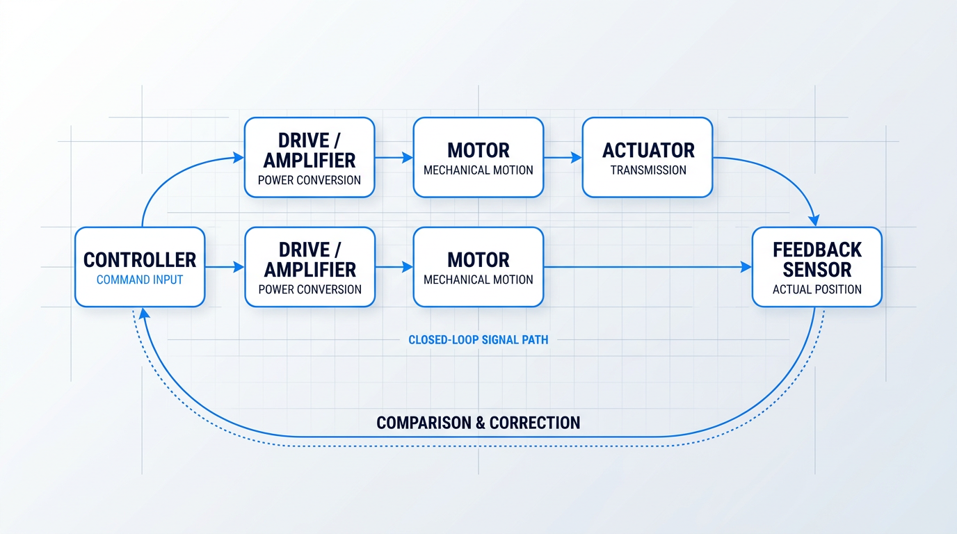
Motion control is not a single device — it is a system of interacting subsystems, each with a defined role, working in concert to translate a command into controlled physical movement.
- Controller: The decision-making layer. Receives input commands, executes motion algorithms, and issues output commands to the drive.
- Drive / Amplifier: The power-conversion layer. Translates low-level controller commands into the precise electrical output needed to energise the motor.
- Motor: Converts electrical energy into mechanical motion — either rotary or linear — as directed by the drive.
- Actuator / Mechanical Transmission: Converts motor output into the specific motion the application requires: linear travel, rotary indexing, or otherwise.
- Feedback Sensor: Measures the actual motion of the load and reports it back to the controller or drive for comparison against the command.
These five subsystems are connected in a defined signal path: a motion command originates in the controller, is amplified and conditioned by the drive, executed mechanically by the motor and actuator, and then verified by the feedback sensor.
The loop closes when the controller compares the commanded motion against the actual motion reported by the sensor — and issues a correction if there is any error between the two.
The fundamental unit of this system is the axis — one degree of freedom, governed by one motor, one drive, and one set of feedback and control hardware.
Real-world machines rarely operate on a single axis: a robot arm coordinates six or more, a CNC machining centre typically manages three to five, and a pick-and-place system may synchronise several axes simultaneously to achieve complex, compound motion.
In motion control, precision and repeatability outrank raw speed. A system that moves fast but inconsistently will produce defects at high volume; one that is slower but repeatable will hold tolerance across millions of cycles. Evaluate motion control systems on consistency first.
Knowing what a motion control system is made of is the necessary first step; understanding how it decides whether the commanded motion was actually executed — and what it does when it was not — is the next.
Open-loop vs. Closed-loop Control: The Foundational Choice
Before you select a motor, size a drive, or specify a feedback sensor, one architectural decision shapes every other choice in a motion control system: whether the control loop is open or closed.
Open-loop control: command without confirmation
In an open-loop system, the controller issues a command — a pulse train, a voltage reference, a digital setpoint — and the signal travels one way: through the drive, to the motor, to the load.
Nothing comes back. There is no feedback path, no measurement of what the actuator actually did, and no mechanism to detect or correct errors.
The system operates on the assumption that the commanded motion was executed — an assumption that holds only as long as the load, speed, and environment stay within the bounds the system was designed around.
Closed-loop control: measure, compare, correct
A closed-loop system adds a feedback sensor to the signal path: the sensor measures the actual output — position, velocity, or torque — and reports it back to the controller continuously.
The controller compares that measured value to the commanded setpoint, calculates the error, and issues a correction — then the cycle repeats.
This is the "loop" in closed-loop: the signal path runs from controller to drive to motor to sensor and back to controller, forming a closed circuit rather than a one-way chain.
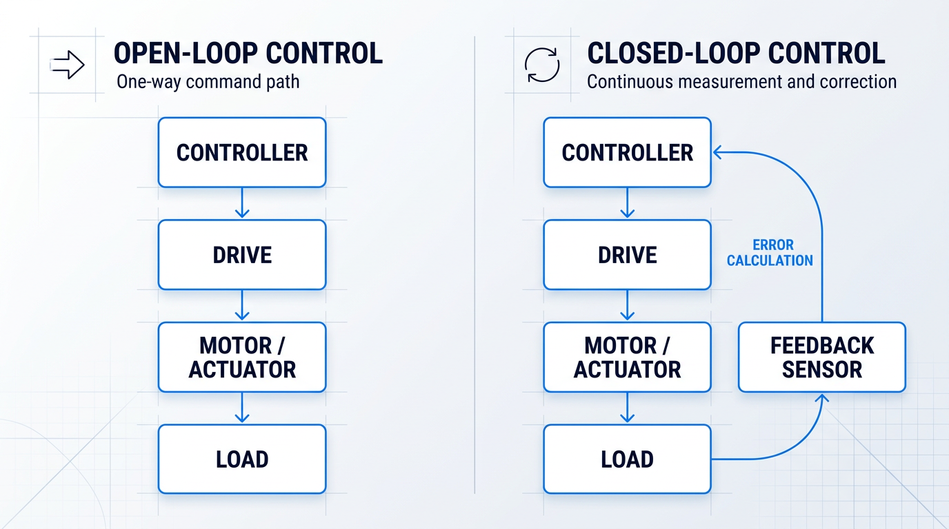
The trade-off between these two architectures is a genuine engineering decision, not a hierarchy where one is always superior.
- Predictable, stable load: The driven load does not change unexpectedly during operation, so the motor always works within its rated capability.
- Modest accuracy requirements: The application tolerates small positional or velocity errors — exact repeatability is not a process-critical requirement.
- Controlled environment: Temperature, friction, and mechanical compliance are stable enough that disturbances will not cause the motor to miss steps or stall.
- Cost-sensitive, low-stakes operation: Adding sensors, wiring, and loop-tuning effort would cost more than the precision gain is worth — a label dispenser or basic indexing table, for example.
When all four of these conditions are met, open-loop is a sound engineering choice: simpler to commission, lower in hardware cost, and free of the loop-tuning complexity that closed-loop systems require.
The moment any condition is violated — load varies unpredictably, accuracy matters, or the environment introduces disturbances — the case for closed-loop feedback becomes compelling.
Without a feedback path, a motion control system cannot verify that the commanded motion was actually executed. In any precision or safety-relevant application, that gap is not a trade-off to manage — it is an unacceptable risk.
In practice, closed-loop is the standard for serious industrial motion control precisely because real applications rarely stay inside the clean boundaries that make open-loop reliable.
A servo axis drifting under thermal expansion, a drive overshooting due to an inertia mismatch, a motor stalling under an unexpected load spike — none of these faults are detectable or correctable without a feedback sensor in the loop.
Feedforward: pre-compensating before error occurs
Feedforward control is a third strategy that experienced engineers apply when an application demands both high speed and high accuracy.
Rather than waiting for the feedback loop to detect an error and issue a correction, feedforward uses a mathematical model of the process — accounting for inertia, friction, and expected load profile — to pre-compensate the command signal before the error can develop.
In practice, feedforward is almost always paired with closed-loop error correction: the feedforward term handles the predictable, model-based component of the required output, while the feedback loop handles residual errors and real-world disturbances the model did not anticipate.
Stepper motors: the open-loop position control exception
Stepper motors occupy a unique position in the motion control landscape: they are the only common motor technology capable of position control without a feedback sensor.
Because a stepper moves in fixed, discrete angular increments, the controller can track commanded position simply by counting the pulses it has issued — no encoder required to confirm where the shaft actually is.
The limitation is a silent failure mode: if the motor misses steps under overload, the controller's internal count diverges from the shaft's true position, and the system has no way of knowing.
Closed-loop stepper systems — steppers fitted with encoders — exist precisely to close this gap, combining the simplicity and cost advantages of stepper drives with the verification capability of closed-loop feedback.
With the open-loop and closed-loop architectures established, the next question is what hardware implements them — specifically the two layers that translate a motion command into physical motor action: the controller and the drive.
Controllers and Drives: Command and Power Layers
Every motion control system depends on two inseparable hardware layers: a motion controller that decides what movement to make, and a drive that delivers the electrical power to make it happen — and neither is useful without the other.
The controller: the decision-making layer
The motion controller is the brain of the system: it receives input signals from operators, process triggers, and feedback sensors, then executes motion algorithms — trajectory generation, PID calculations, multi-axis interpolation — and issues precise commands to the drives.
Three main hardware categories exist, each suited to a different application profile and design constraint.
- Dedicated motion controllers: Purpose-built for real-time trajectory generation and multi-axis coordination; typically DSP or FPGA-based for deterministic, high-performance motion tasks.
- PLCs with motion capability: General-purpose industrial controllers extended with motion function blocks under the PLCopen standard; best when motion is one part of a broader machine control task.
- Drive-integrated controllers: Controller intelligence embedded directly inside the drive unit, eliminating a separate hardware layer; common in single-axis and compact multi-axis applications.
The industry is accelerating toward a further step: combining the servo motor, drive, controller, and feedback device into a single intelligent package — sometimes called a smart drive or integrated servo system.
The engineering case for this integration is concrete: it reduces wiring harness complexity, eliminates communication latency between the controller and drive, simplifies commissioning, and shrinks cabinet footprint — a genuine architectural shift for compact and distributed multi-axis applications.
Connecting the controller to the drive has its own infrastructure story: older systems relied on ±10 V analogue signals — simple, but bandwidth-limited, noise-susceptible, and incapable of carrying diagnostic data.
Modern systems use digital industrial fieldbuses — EtherCAT, EtherNet/IP, and Modbus TCP are the dominant protocols — with EtherCAT the established standard for demanding motion applications where tight multi-axis synchronisation is required.
Latency in the communication path between controller and drive directly degrades positioning accuracy. Real-time deterministic fieldbuses are foundational infrastructure for closed-loop motion control — not an optional upgrade.
The drive: power conversion and loop closure
The drive receives a command from the controller — a position setpoint, velocity reference, or torque demand depending on control mode — and converts it into the precise voltage and current waveforms the motor requires.
Critically, a drive is not merely a power amplifier: most drives close one or more control loops internally, which is why the choice of drive type and control mode shapes the dynamic behaviour of the entire motion system.
A servo drive implements three nested control loops, each running at a different bandwidth: the innermost current (torque) loop regulates motor phase current at tens of kHz; the velocity loop sits outside it and regulates speed at a few kHz; the outermost position loop compares commanded position to actual position from the feedback device and commands a velocity setpoint inward.
Which loops are active depends on the operating mode: torque mode closes only the current loop; velocity mode closes current and velocity; position mode activates all three — making servo drives the right choice for precision positioning applications with high dynamic response requirements.
A stepper drive works differently: it issues discrete electrical pulses to the motor windings, advancing the rotor by a fixed angular step per pulse, and operates open-loop by default — the drive assumes each commanded step was executed with no position verification.
This simplicity makes stepper drives lower-cost and tuning-free, but the trade-off is real: if the motor misses a step under overload, the error accumulates silently. Closed-loop stepper drives with encoder feedback address this gap, though at added cost.
A variable frequency drive (VFD) serves a different purpose entirely: it controls AC induction motor speed by varying the output frequency and voltage, and offers three levels of control sophistication.
- V/Hz (Volts-per-Hertz): Simplest method; maintains a fixed voltage-to-frequency ratio. Adequate for fans, pumps, and conveyors where speed precision is not critical.
- Sensorless vector control: Uses a motor model to estimate flux and torque without a shaft encoder; delivers better speed regulation under varying load than V/Hz.
- Closed-loop vector / FOC: Field-oriented control with a shaft encoder for precise flux and torque management; highest VFD precision, approaching servo-like performance in some applications.
VFDs are the right tool when speed control of AC induction motors is the requirement — but they are not a substitute for servo drives where precise position control or high dynamic response is demanded.
With the controller and drive layers established, the natural next question is what the drive is actually energising — which brings us to the motors themselves.
Motors: Where Electrical Power Becomes Motion
The drive delivers precisely conditioned electrical power — but it is the motor that determines what the system can actually do with it, setting the torque-speed ceiling, the feedback architecture, and ultimately the performance limits of the entire motion control system.
Motor selection is therefore not a downstream detail; it is one of the earliest and most consequential decisions in system design, because the motor type constrains every component choice that follows.
Servo Motors: The Precision Workhorse
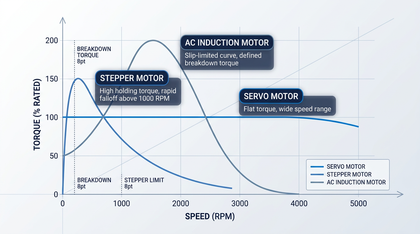
The servo motor is the default choice for precision industrial motion control, and for good reason: it combines high torque density with a flat torque curve across a wide speed range, fast dynamic response, and closed-loop positioning capability.
Critically, the servo motor and its feedback device are a unified system — the encoder is built into the motor, and that integration is what closes the loop described in §4.
Modern industrial servo motors are almost universally brushless AC designs, which means mechanical commutation has been eliminated entirely, removing the brush wear and debris that limited earlier DC servo designs.
The result is a motor that suits any application demanding high speed, rapid dynamic response, and verified precise positioning — paired with a servo drive, it forms the most capable drive-motor combination available in standard industrial practice.
Linear and Direct-Drive Servo Variants
The linear servo motor extends the servo concept to produce direct linear force without any mechanical transmission — delivering the highest achievable linear speed and acceleration, zero backlash, and no mechanical wear in the drive train.
The engineering trade-off is thermal: linear motors generate significant heat under high-force operation, and demanding applications typically require secondary cooling to sustain performance.
The direct-drive rotary servo motor couples the load directly to the rotor and eliminates the gearbox entirely — removing gearbox backlash, torsional flex, and the mechanical compliance that limits servo tuning performance in geared systems.
Many direct-drive designs offer a hollow-bore rotor, which simplifies cable routing through the axis — a practical integration advantage in semiconductor handling, CNC 4th and 5th axes, and precision indexing tables where stiffness and backlash-free operation justify the higher motor sizing requirement.
Stepper Motors: Open-Loop Positioning at Lower Cost
The stepper motor operates on a fundamentally different principle: it is a brushless DC motor that advances in fixed angular increments, typically 1.8° per step, giving 200 full steps per revolution.
This discrete-step architecture delivers excellent holding torque at standstill and high torque at low speeds, requires no tuning, and costs significantly less than a comparable servo system.
The limitation is equally fundamental: torque falls off sharply as speed increases, and because stepper motors are the canonical open-loop positioning technology (as discussed in §4), the system has no means to detect or recover from a missed step under overload.
Closed-loop stepper variants address this verification gap by adding feedback, but the underlying torque-speed curve remains a constraint — the stepper's niche is low-speed, cost-sensitive positioning where the load profile is well-characterised and predictable.
AC Induction Motors: The Industrial Volume Workhorse
The AC induction motor dominates industrial applications where precision positioning is not the requirement — and it dominates for straightforward reasons: simple construction, exceptional ruggedness, low cost, high standardisation, and availability across virtually every power rating.
Speed is determined by supply frequency and pole count, with a small slip between synchronous and actual rotor speed — a characteristic that also defines the motor's natural torque-speed curve and its breakdown torque limit.
As covered in §5, AC induction motors are what variable-frequency drives power: the VFD adjusts supply frequency to vary speed, enabling controlled operation in fans, pumps, conveyors, and similar constant-load applications without the cost or complexity of a servo system.
DC Motors: Brushed and Brushless
DC motors offer an intrinsically straightforward control relationship: speed is proportional to applied voltage, and torque is proportional to current — which made them the first motor type widely used in variable-speed industrial drives.
Brushed DC motors achieve commutation mechanically via brushes and a commutator, which introduces a wear item that generates carbon debris and demands periodic maintenance — a meaningful operational cost in continuous industrial use.
Brushless DC (BLDC) motors move commutation into electronics, preserving the controllability of DC while eliminating the mechanical wear point entirely.
Modern brushless DC servo motors represent the convergence of DC's linear control relationships with brushless reliability — which is why they now dominate precision motion applications and are the motor technology underlying most contemporary servo systems.
Comparing the Four Types: Selection Trade-offs
Each motor type occupies a distinct position across the axes that matter most in practice: torque-speed profile, positioning capability, drive pairing, and cost tier.
| Motor Type | Torque-Speed Profile | Positioning Capability | Typical Drive Pairing | Cost Tier | Primary Application Contexts |
|---|---|---|---|---|---|
| Servo motor (brushless AC) | Flat torque across wide speed range; high torque density | Closed-loop absolute; encoder built in | Servo drive | High | Precision positioning, robotics, CNC axes, packaging |
| Stepper motor | Peaks at low speed; falls sharply above ~1,000 RPM | Open-loop incremental; 1.8° per step (200 steps/rev); no missed-step detection | Stepper drive (pulse/direction) | Low–medium | Low-speed positioning, label applicators, 3D printing |
| AC induction motor | Slip-limited curve; defined breakdown torque at ~200–300% rated | Speed regulation only; no inherent positioning | Variable-frequency drive (VFD) | Low | Fans, pumps, conveyors, compressors |
| DC motor (brushless) | Linear speed-voltage, torque-current relationship; wide speed range | Closed-loop with external feedback; high controllability | DC servo drive or BLDC drive | Medium–high | Precision servo applications, mobile robotics, spindles |
Comparison of the four primary motor types across key selection axes to support engineering motor selection decisions.
The table reveals a clear pattern: servo motors lead on every performance axis but carry the highest cost, while AC induction motors and steppers occupy the cost-efficient end at the expense of positioning capability and dynamic response.
The stepper's open-loop 1.8° step increment looks attractive until the load becomes unpredictable — at which point the inability to verify position becomes a reliability liability that a servo system eliminates by design.
No single motor type wins across torque-speed profile, feedback architecture, and cost simultaneously. The right choice is the one that satisfies the application's minimum requirements on all three axes — not the highest-performing motor the budget can stretch to.
Producing rotation — or direct linear force in the case of linear motors — is only half the story: the next question is how that output is converted into the specific motion the application actually needs, whether that is linear travel, geared rotation, or direct drive of a load.
Once the motor produces its output, the system still needs to convert that force or rotation into the specific mechanical motion the application demands — which is where actuators and transmission elements take over.
Actuators and mechanical transmission: converting motor output
The motor shaft rotates — but the application needs a carriage to travel 800 mm along a linear axis, or a rotary table to index to within an arc-second, or a robot joint to swing through a precise angle under load. The gap between what a motor produces and what the machine actually needs is bridged by actuators and the mechanical transmission elements that connect them to the load.
Actuators divide into two fundamental families: rotary actuators, which produce rotational motion for applications such as valve operation, indexing tables, and robot joints, and linear actuators, which produce motion along a straight line for lifting, positioning, pushing, and clamping.
Most linear actuators in precision industrial motion control do not generate linear motion directly — they convert the rotary output of a motor into linear displacement via a mechanical transmission. The choice of transmission technology is one of the most consequential decisions in a motion system design, because it determines the achievable precision, maximum speed, practical stroke length, and maintenance burden of the entire axis.
Linear transmission technologies compared
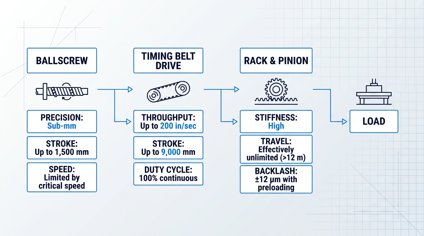
Three technologies dominate precision linear motion in industrial automation: ballscrews, timing belt drives, and rack and pinion drives. Each occupies a distinct performance envelope, and the right choice depends on the specific demands of the application.
| Technology | Mechanical Efficiency | Typical Stroke Range | Duty Cycle |
|---|---|---|---|
| Ballscrew | 80–95% | Up to ~5 ft (1,500 mm) typical | Moderate — critical speed limits high-speed long-stroke use |
| Timing Belt Drive | 90–93% | Up to ~30 ft (9,000 mm) | 100% — no critical speed limitation |
| Rack and Pinion | Up to 97% | Effectively unlimited (>40 ft / 12 m) | High — suited to continuous duty long-travel axes |
Comparison of the three main linear transmission technologies across efficiency, typical stroke range, and duty cycle, using figures sourced from Parker Hannifin and Machine Design.
The efficiency figures alone do not tell the full story: each technology excels in a different part of the application space, and selecting purely on efficiency would lead to poor system choices.
Ballscrews: the precision linear standard
A ballscrew converts rotary motor torque into linear force via a threaded shaft and nut with recirculating ball bearings — the rolling contact dramatically reduces friction compared to a plain leadscrew, yielding mechanical efficiencies of 80–95% and highly predictable service life.
For CNC machining centres, precision assembly equipment, and any axis where sub-millimetre positional accuracy and repeatability are non-negotiable, the ballscrew is the standard choice. Its low compliance and well-characterised error budget make it straightforward to integrate into a closed-loop servo system.
The key limitation is critical speed: as stroke length increases or rotational speed rises, the screw shaft can begin to whip and resonate at its natural frequency, degrading positioning performance and risking mechanical damage. The longer and narrower the shaft, the lower the critical speed threshold — which is why ballscrews are most reliably applied in strokes up to around 1,500 mm, and why engineers reach for belt drives or rack and pinion when the application demands more travel.
Timing belt drives: long stroke, high throughput
Timing belt drives use a toothed belt and pulley to convert rotary motor output into linear motion, with efficiencies of 90–93% and no critical speed ceiling. Belt-driven actuators can achieve stroke lengths well beyond 200 inches (5,080 mm) and linear speeds up to 200 inches per second — performance ranges that ballscrews simply cannot reach.
The trade-off is positional accuracy: the belt has inherent compliance, which means timing belt drives cannot match the positional precision of a ballscrew. For high-throughput pick-and-place, material handling, and long-travel gantry axes where cycle rate matters more than absolute positional accuracy, that trade-off is entirely acceptable. Belt drives also support 100% duty cycle operation with minimal maintenance, making them well-suited to continuous production environments.
Rack and pinion: long travel with high stiffness
When stroke length exceeds what a ballscrew can handle reliably and the application still demands high stiffness and good dynamic performance, rack and pinion is the natural choice. Helical rack and pinion drives achieve efficiencies up to 97%, and with effectively unlimited travel length they are the standard solution for large CNC gantry machines, laser cutting tables, and plasma cutting systems.
Backlash has historically been the weakness of rack and pinion, but modern electronic preloading techniques — using a dual-pinion arrangement where a slave pinion generates opposing torque to eliminate tooth clearance — can deliver backlash-free operation across the full travel length. With hardened and ground tooth profiles, cumulative pitch errors as low as ±12 µm over 500 mm are achievable, bringing rack and pinion into contention for genuinely high-precision long-travel axes.
Gearboxes: inertia matching and torque multiplication
A gearbox placed between motor and load does two things: it multiplies output torque in proportion to the gear ratio, and it reduces the speed at the output shaft by the same factor. Both are useful — but the more important function in precision servo applications is often inertia matching.
When a gearbox with ratio N:1 is inserted into the drivetrain, the reflected inertia of the load as seen by the motor is reduced by N². A 5:1 gearbox reduces reflected inertia by a factor of 25 — meaning a load with 25 times the motor's inertia now presents as a 1:1 match at the motor shaft. This is not merely a convenience: for high-performance servo systems, the inertia ratio between load and motor should ideally be kept below 10:1, and a well-chosen gearbox ratio is often the most direct way to achieve that target.
A gearbox with ratio N:1 reduces the load's reflected inertia at the motor shaft by N-squared. A 5:1 gearbox makes a load with 25x the motor's inertia behave as a 1:1 match — critical for achieving stable servo tuning and fast dynamic response.
Planetary gearboxes are the dominant choice for precision servo applications: compact, high torque density, and approximately 97% efficient per stage in a single-stage unit. Their load-sharing architecture — multiple planet gears distributing torque simultaneously — also delivers high torsional stiffness, which is essential for axes subject to frequent direction reversals.
Backlash is the critical precision consideration for any gearbox. A typical planetary gearhead carries 1–9 arc-minutes of backlash; in positioning applications with bidirectional motion, that lost motion translates directly into positioning error at the load. For precision servo applications, zero-backlash or low-backlash gearbox designs — using precision ground gears, reduced centre distances, or split-gear preloading mechanisms — are specified to keep this error within acceptable bounds.
Direct-drive: eliminating the transmission entirely
The logical endpoint of backlash reduction is to remove the gearbox altogether. In a direct-drive actuator, the motor rotor couples directly to the load with no intervening gearing — eliminating backlash, mechanical compliance, and transmission losses in a single step. Direct-drive systems achieve transmission efficiencies approaching 99%, and because there is no gear mesh or belt stretch to introduce hysteresis, servo gains can be set significantly higher than in transmission-based systems.
The cost is that the motor must deliver full load torque natively, at the speeds the application requires — not at the high-speed, low-torque operating point that makes conventional motors compact and efficient. Direct-drive motors are therefore larger, heavier, and more expensive than their geared equivalents: initial cost premiums of 30% or more are typical, rising considerably for frameless designs. The investment is justified when backlash, compliance, and transmission wear are genuinely unacceptable — as they are in semiconductor wafer handling, precision rotary tables, and high-accuracy inspection systems.
Choosing the right transmission: a multi-axis decision
No single transmission technology dominates across all applications. The selection is a multi-axis trade-off: precision requirements, stroke length, speed, force, duty cycle, and maintenance overhead all feed into the decision simultaneously.
- Short stroke, high precision: Ballscrew. The standard choice for CNC machining centres and precision assembly where sub-millimetre accuracy and repeatable positioning are paramount.
- Long stroke, high throughput: Timing belt drive. Ideal for pick-and-place, material handling, and continuous-duty axes where speed and stroke length outweigh absolute positional accuracy.
- Long travel, high stiffness: Rack and pinion. The correct step-up from ballscrews on large gantries, laser tables, and plasma cutters; precision need not be sacrificed with preloading.
- Torque multiplication and inertia matching: Planetary gearbox. Converts high-speed, low-torque motor output and reduces reflected inertia by N-squared to achieve stable servo tuning.
- Zero backlash, maximum stiffness: Direct-drive. Removes the transmission entirely; the right choice when backlash and compliance are genuinely unacceptable, at a higher motor cost.
A ballscrew is not universally superior to a belt drive — it is simply the right tool for a different application envelope. The engineer's job is to identify which performance dimensions the application cannot compromise on, and let those constraints drive the selection.
With the transmission chosen and the motion delivered to the load, the control loop still has one question left to answer: did the axis actually move to where it was commanded? That question is the territory of feedback devices — encoders, resolvers, and linear scales — which form the subject of the next section.
Feedback Devices: Closing the Loop
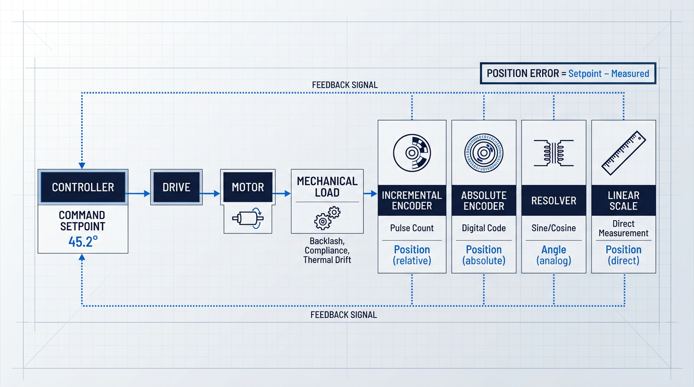
The mechanical chain from motor to load — covered in the previous section — produces motion, but it cannot verify it. That verification is the job of the feedback device: a sensor or transducer that converts shaft rotation or linear displacement into electrical signals the controller or drive can read, compare against the commanded setpoint, and act on.
The difference between the commanded position and the measured position is the position error. Eliminating that error, continuously and in real time, is what closed-loop control means in practice — and no amount of controller sophistication changes the fact that the loop cannot close without a feedback device to sense what the load is actually doing.
Incremental encoders
Incremental encoders generate a stream of pulses as the shaft rotates — typically from a optical disc with alternating transparent and opaque segments, or a magnetic ring with alternating poles. Position is determined by counting those pulses from a known reference point, usually an index mark on the encoder disc.
They are the workhorse of industrial servo systems: mechanically simple, cost-effective, and supported natively by virtually every drive and motion controller platform on the market.
The engineering trade-off is the homing requirement. Because an incremental encoder measures position relative to a reference, the system must execute a homing cycle at startup to establish where it is. If power is lost mid-cycle, that reference is gone and homing must be repeated. For most applications, this is entirely acceptable — the homing cycle takes seconds and relative position feedback is all the application needs.
Absolute encoders
Absolute encoders assign a unique digital code to every shaft position across the full range of travel, so the encoder always knows exactly where it is — even immediately after power-up, and even after an unplanned power loss or emergency stop.
The cost premium over incremental encoders is real, but increasingly easy to justify. Safety-critical applications cannot afford the time or risk of a homing cycle after an e-stop; high-uptime production lines cannot absorb the restart delay; and as absolute encoder technology has matured, the price gap has narrowed considerably. For serious industrial servo applications, absolute encoders are becoming the default rather than the premium option.
Resolvers
A resolver is an electromechanical transducer built on transformer principles: a rotor winding couples inductively with two stator windings arranged in quadrature, and the relative amplitude of the two output signals encodes shaft angle. There are no onboard electronics — no photodetectors, no ASICs, no silicon of any kind.
That absence of electronics is the resolver's defining engineering property. It makes resolvers extraordinarily tolerant of high temperature, mechanical shock, vibration, contamination, and electromagnetic interference — conditions that would degrade or destroy silicon-based encoder electronics. The trade-off is that the analog sine/cosine output requires a resolver-to-digital (R/D) converter in the drive or a dedicated interface module, which adds cost and a layer of signal-chain complexity.
Where resolvers earn their place is in genuinely harsh environments: aerospace actuators, defence systems, heavy industrial machinery, and downhole oil and gas equipment — applications where an encoder's electronics would fail or demand frequent replacement.
Linear encoders and scales
Every rotary encoder — whether incremental, absolute, or resolver-based — mounted on a motor shaft measures rotation and infers linear position at the load through the transmission geometry. A linear encoder takes a fundamentally different approach: it measures displacement directly at the load, along the axis of motion.
This distinction matters because the transmission between motor shaft and load is never perfect. Mechanical compliance, backlash, thermal expansion, and wear all introduce position error that a rotary encoder on the motor cannot see — but a linear scale mounted at the load measures through all of it.
The applications where this matters most are those where the transmission itself is a meaningful error source: high-accuracy CNC machining centres (where thermal growth of the ballscrew between motor and tool tip is a real, measurable effect), and semiconductor wafer-handling stages where nanometre-level positioning is required. For any linear axis where the highest achievable accuracy is the goal, direct linear feedback is the path to get there.
Feedback accuracy and servo performance
The choice of feedback device is not a secondary specification — it sets the performance ceiling for the entire servo system. A servo loop can only correct errors it can detect, and it can only detect errors the feedback device can resolve.
Higher-resolution feedback enables tighter servo tuning: higher proportional gains become stable, the control loop can run at greater bandwidth (issuing more corrections per second), and the system can detect and reject smaller disturbances before they accumulate into position error. Conversely, low-resolution or noisy feedback forces the engineer to back off the gains — the controller cannot distinguish genuine position error from quantisation noise, and an aggressively tuned loop will oscillate.
The servo system is only as accurate as the feedback it receives. No amount of controller sophistication can recover positional accuracy that the feedback device cannot see — feedback selection is a system-level engineering decision, not an afterthought.
The highest-performance configuration takes this logic to its conclusion: a dual-encoder setup, with one encoder on the motor shaft for commutation and velocity loop closure, and a second encoder or linear scale mounted directly on the load for position loop closure.
This architecture means the position loop is closed on actual load position, not inferred load position — so mechanical compliance, backlash, and thermal growth between motor shaft and load are eliminated as error sources for the position loop. It requires a drive or controller with dual-feedback inputs, and adds cost and integration complexity, but for precision machine tools, semiconductor stages, and metrology equipment, it is the configuration that makes the highest accuracy targets achievable.
With the feedback device families understood — what they measure, how they differ, and how their accuracy shapes loop performance — the natural next question is how that performance is specified, measured, and evaluated at the system level, which is what the following section addresses.
Specifying and connecting a motion control system
Selecting the right motor, drive, actuator, and feedback device is the tractable part of a motion control project — the part that shows up in datasheets and procurement lists. What determines whether the assembled system actually performs is harder to specify: how well the components are tuned together, how reliably the communication network delivers data within every control cycle, and how the system behaves under real production load.
Accuracy, repeatability, and resolution
Accuracy and repeatability are frequently conflated, but they describe fundamentally different things. Accuracy is how close the system gets to the commanded absolute position; repeatability is how consistently it returns to the same position across successive cycles.
In most production environments, repeatability is the more operationally critical parameter. A system with a consistent positional offset can be compensated for in software or through calibration; a system that lands in a different place each cycle cannot be corrected for, because the error has no predictable pattern.
A consistent offset is correctable. Cycle-to-cycle variation is not. When specifying a motion system for production, prioritise repeatability first — accuracy can often be calibrated in; inconsistency cannot be engineered out.
Resolution — the smallest incremental movement the system can command — is set by the feedback device's resolution and the drive's interpolation capability. But high resolution does not guarantee high accuracy.
If mechanical compliance, backlash, or thermal growth absorbs small commanded increments, the system cannot execute them regardless of how finely the encoder resolves position. As Parker's linear drive train data shows, a linear motor can achieve sub-micron resolution and repeatability, while a timing belt system with equivalent encoder resolution may deliver only ~50 µm repeatability — the mechanical transmission, not the encoder, is the limiting factor.
Dynamic response, loop bandwidth, and inertia matching
Loop bandwidth, expressed in Hz, describes how quickly the control loop can respond to a command change or reject a disturbance. Higher bandwidth means faster settling after a move and better resistance to external disturbances such as vibration or load variation — both critical in high-speed or high-precision applications.
What limits loop bandwidth in practice is a combination of mechanical resonance in the load, inertia mismatch between motor and load, and communication latency in the control loop. Mechanical resonance sets a ceiling: servo bandwidth must stay well below the system's resonant frequency to avoid exciting oscillation, which is why notch filters are a standard commissioning tool for suppressing specific resonant frequencies and recovering bandwidth.
Inertia matching — the ratio of load inertia to motor inertia — directly shapes dynamic performance and how readily the servo loop can be tuned. A ratio close to 1:1 is the theoretical ideal for maximum power transfer and loop stability; as Yaskawa's sizing guidance notes, ratios of 5:1 are typical for many applications, while ratios above 10:1 make quick positioning increasingly difficult and cause the load to overshoot and oscillate before settling.
When load inertia is high, a gearbox is the standard remedy: as covered in the actuators section, reflected inertia is reduced by the square of the gear ratio, so even a modest reduction provides significant inertia management without requiring a larger motor.
Real-time communication: the infrastructure layer
Communication latency is not a network administration concern — it is a positioning accuracy concern. The controller cannot correct an error it has not yet been told about, so every microsecond of latency between a feedback device reporting position and the controller issuing a correction is a window during which the system is running open-loop. For demanding motion control applications, real-time communication is foundational infrastructure, not an optional upgrade.
Three protocols dominate industrial motion control networks, each with distinct performance characteristics suited to different application tiers.
| Protocol | Minimum Cycle Time | Synchronisation Jitter | Typical Application |
|---|---|---|---|
| EtherCAT | 100 µs for 100 servo axes; sub-100 µs achievable | Much less than 1 µs (measured ~±20 ns at 300 nodes) | Demanding multi-axis motion, high-speed pick-and-place, semiconductor equipment |
| PROFINET IRT | 31.25 µs with Conformance Class C hardware | Less than 1 µs | High-precision motion in Siemens-ecosystem machines; packaging, printing, CNC |
| CANopen | ~10 ms SYNC interval typical; single frame ~55 µs at 1 Mbit/s | Not specified to sub-millisecond; varies with bus load | Lower axis-count applications, embedded systems, distributed I/O |
Comparison of the three primary industrial motion control protocols on cycle time, synchronisation jitter, and typical application scope
EtherCAT is the benchmark for demanding multi-axis motion: the EtherCAT Technology Group confirms cycle times of 100 µs or less and synchronisation jitter well under 1 µs, with measurements showing approximately ±20 ns across 300 nodes. Its on-the-fly frame processing architecture — where each node reads and inserts data as a single frame passes through — means cycle time scales efficiently regardless of node count.
PROFINET IRT achieves cycle times down to 31.25 µs with jitter below 1 µs through hardware-based bandwidth reservation and scheduled switching, making it the natural choice in Siemens-ecosystem machine builds where tight axis synchronisation is required. CANopen remains widely supported and well-suited to lower axis-count or less timing-critical applications, but its 1 Mbit/s physical layer and SYNC-based timing architecture place it in a different performance tier from the industrial Ethernet protocols.
Multi-axis coordination and commissioning
Multi-axis systems are not simply multiple single-axis systems running in parallel. Synchronisation, interpolation, electronic gearing, and camming all require the controller to execute real-time calculations across axes simultaneously — and each adds a layer of complexity that concentrates in the controller and the communication network.
As Control Engineering's analysis of synchronised motion confirms, interpolation — where two or more axes follow a coordinated path with continuously recalculated velocity and acceleration vectors — is the most complex coordination mode, requiring the controller to look ahead and proactively adjust path velocity to avoid axis limit violations. Electronic gearing and camming (where one axis slaves to another via a fixed ratio or programmable cam profile) are less computationally intensive but still require deterministic communication to maintain phase relationships across every cycle.
The honest reality of commissioning a multi-axis motion system is that it is a substantial engineering task, routinely underestimated at the project planning stage. Setting PID gains, feedforward terms, and notch filters for each axis; configuring the communication network; managing axis interdependencies; and validating performance under real production load conditions — each demands skilled engineering time that does not appear in a hardware bill of materials.
Hardware selection is the visible, tractable part of a motion control project. Getting the system to communicate reliably, tune correctly, and perform consistently under production conditions is where real-world projects succeed or fail — and the engineering effort required is almost always larger than the initial estimate.
With the evaluation framework established, the practical question becomes: what do these performance demands actually look like when a motion control system is deployed in a specific industry? The next section examines exactly that, across robotics, CNC machining, semiconductor fabrication, pharmaceutical manufacturing, and aerospace.
Motion control in practice: key industrial applications
The components and architectures covered in earlier sections don't exist in a vacuum — they exist because real industries impose real engineering problems that cannot be solved any other way. Each of the five applications below places a distinct combination of demands on the motion control system, and understanding those demands is what separates a system that works from one that merely moves.
Robotics: coordinated multi-axis motion in real time
Every joint of an articulated robot arm is a controlled axis, and the controller must coordinate all of them simultaneously to execute smooth, accurate paths through space — this is the defining motion control challenge in robotics.
Servo motors are the standard choice at each joint, with high-resolution feedback devices closing the loop and giving the controller the positional data it needs to execute kinematics calculations in real time.
Those kinematics calculations are computationally demanding: inverse kinematics must be solved within the servo loop cycle time, which means the controller's real-time processing capability is not a nice-to-have — it is a hard system requirement.
Collaborative robots (cobots) operate at lower stiffness and accept more compliance to enable safe human co-working, which means their repeatability requirements are less stringent than those of traditional industrial robots.
Traditional industrial robots, by contrast, are designed for rigid, high-repeatability fixed automation where positional consistency across thousands of cycles is the primary metric — and the servo system must be specified accordingly.
A concrete illustration of how precision motion enables repeatable industrial processes: automated laser cleaning cells mounted on robotic arms must return to exactly the same surface geometry on every cycle to deliver consistent results — the motion system is what makes that repeatability achievable at production speed.
CNC machining: interpolation accuracy and surface finish
CNC machining is one of the most unforgiving motion control environments for positional accuracy: any error in the controller's interpolation across X, Y, Z and rotary axes translates directly into dimensional error or surface finish degradation on the finished part.
The standard approach to eliminating transmission error is mounting high-resolution linear encoders directly at the load rather than inferring position from motor shaft rotation — the dual-encoder and linear scale approach discussed in the feedback devices section exists precisely because ballscrew and gearbox compliance would otherwise introduce error that the motor-side encoder cannot see.
At high feed rates, mechanical resonance in the machine structure becomes a significant source of surface finish degradation. Servo drives with vibration suppression algorithms — typically implemented as notch filters tuned to the machine's resonant frequencies — are used to attenuate these effects and maintain surface quality without reducing feed rate.
The motion control layer forms the foundation of a CNC machining system: coordinated multi-axis interpolation and path accuracy directly determine what geometries the machine can hold in production, which is why the controller and drive architecture cannot be treated as commodity selections.
Semiconductor manufacturing: nanometre-scale positioning
Semiconductor manufacturing sits at the extreme end of the motion control precision spectrum: wafer alignment, lithography, and inspection processes require positional accuracy in the micrometre-to-nanometre range, well beyond what standard industrial servo systems can deliver.
The actuator technology reflects this: direct-drive linear stages and voice-coil actuators eliminate the mechanical transmission elements — ballscrews, gearboxes, couplings — that introduce backlash and compliance at conventional precision levels.
At this precision level, absolute encoders are supplemented or replaced by laser interferometers, which measure displacement using the wavelength of light and provide resolution that encoder-based systems cannot match.
Vibration isolation and thermal compensation are not optional add-ons at nanometre scale — they are primary engineering constraints. Ambient floor vibration and thermal expansion of the machine structure are error sources of the same order of magnitude as the positioning target, so both must be actively managed as part of the system design.
Cleanroom compatibility adds a further constraint throughout the motion system: linear guides, actuator housings, and lubricants must all be qualified for the particle emission requirements of ISO Class 3–6 cleanroom environments, as certified linear motion technology from suppliers such as Bosch Rexroth demonstrates.
Pharmaceutical manufacturing: synchronisation and regulatory compliance
Filling, capping, and assembly operations in pharmaceutical manufacturing are multi-axis synchronisation challenges: the controller must coordinate multiple axes with precise timing across filling, inspection, and packaging stations, all running at industrial speed.
Planar motor systems — magnetically levitated movers travelling freely over a 2D track surface — are increasingly used for product handling in pharmaceutical lines because each mover can be independently positioned, accelerated, and decelerated, enabling flexible production of multiple SKUs on a single line without mechanical changeover.
Beckhoff's XPlanar system achieves repeat accuracy of ≤5 µm in X, Y, and Z axes with six degrees of freedom per mover — positioning precision that enables the transport system itself to handle product orientation during processing, not just move products between stations.
The defining characteristic of pharmaceutical motion control, however, is that mechanical performance is only half the requirement. GMP validation, 21 CFR Part 11 compliance in the US context, and equivalent EU GMP Annex 11 requirements are system-level design constraints: they shape controller selection, mandate audit trail capabilities, define data logging architecture, and determine how electronic records and signatures must be handled throughout the system.
In pharmaceutical motion control, GMP and 21 CFR Part 11 requirements determine controller selection, data logging design, and audit trail architecture from the outset — they cannot be retrofitted onto a system designed without them.
A motion controller that cannot produce a compliant audit trail of every axis movement, parameter change, and operator intervention is not a viable option in this environment, regardless of its mechanical performance.
Aerospace: manufacturing precision and in-service actuation
Aerospace presents two distinct motion control contexts that place very different demands on the system — one on the factory floor, one in the aircraft itself.
On the manufacturing side, robotic drilling and fastening for aircraft assembly requires positional accuracy of ±0.25 mm or better to achieve correct hole geometry and fastener alignment in composite and metallic airframe structures. Electroimpact's documented work demonstrates that achieving this tolerance requires secondary position feedback mounted at the output of each robot axis — not at the motor shaft — combined with high-order kinematic models to compensate for deflection in the robot's links and bearings.
Standard off-the-shelf industrial robots are practically limited to ±0.5 mm global positional accuracy; the ±0.25 mm aerospace requirement is only achievable with the secondary feedback and kinematic compensation architecture described above — a direct application of the closed-loop principles established earlier in this guide.
On the in-service side, the shift from conventional hydraulic systems to electrohydrostatic actuators (EHAs) and electromechanical actuators (EMAs) for flight control surfaces is driven by weight reduction and reliability requirements, replacing centralised hydraulic circuits with electrically powered actuation at each control surface.
The environmental envelope for in-service aerospace motion systems is extreme: temperature ranges from -55°C to 200°C, combined with severe shock and vibration loads, impose component selection constraints that differ fundamentally from industrial practice. Brushless DC motors are preferred over brushed types for their reliability and maintenance profile in these conditions.
Feedback device selection follows the same environmental logic: resolvers are widely regarded in aerospace engineering practice as more robust than optical encoders under wide temperature swings and sustained vibration, though this preference is grounded in established domain knowledge rather than a single traceable specification.
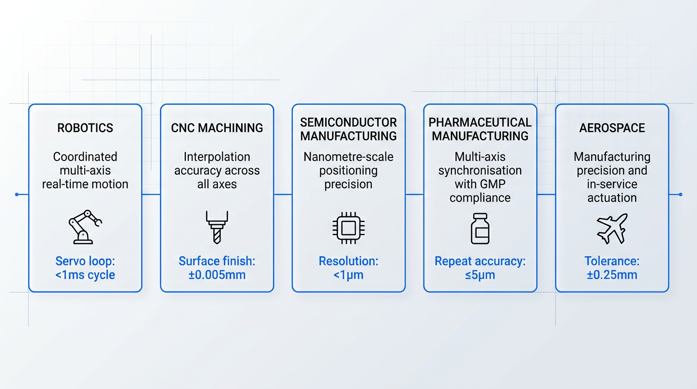
The aerospace application makes explicit what is true across all five industries covered here: environmental constraints, not just precision requirements, shape component selection — and neither can be addressed in isolation from the other.
Across robotics, CNC machining, semiconductor manufacturing, pharmaceuticals, and aerospace, the pattern is consistent: the application imposes a specific combination of precision, speed, environmental, safety, and regulatory demands, and the motion control system must be designed as an integrated whole to meet them. No single component decision — motor type, feedback device, controller platform — can be made without reference to the full set of application requirements, because each choice constrains the others.
The integration complexity these applications create — and the cost of getting it wrong — is precisely what is driving the adoption of AI-enabled tuning, IIoT diagnostics, and Industry 4.0 connectivity tools, which the next section examines in detail.
AI, IIoT, and Industry 4.0 in Motion Control
The engineering challenges established throughout this guide — the commissioning burden of complex multi-axis systems, the cost of unplanned downtime in high-utilisation production, the overhead of managing distributed operations — are precisely the problems that AI-enabled tools, IIoT connectivity, and Industry 4.0 integration are being built to address.
That framing matters. These technologies are gaining traction in motion control not because they are novel, but because the underlying pain points are real and the engineering case for addressing them is increasingly compelling.
AI-enabled adaptive tuning and anomaly detection
Manual servo tuning of complex multi-axis systems has always demanded significant engineering time — and the more dynamic the application, the harder it is to hold those parameters stable as the system ages, loads shift, or mechanical wear accumulates.
Machine learning models integrated directly into the control environment can now analyse motor current signatures, vibration data, and time-series process signals in real time to detect deviations from learned normal behaviour — catching anomalies such as bearing damage, imbalance, or tool wear before they become failures.
Beckhoff's TwinCAT 3 Machine Learning platform exemplifies this approach: ML inference runs directly within the TwinCAT runtime on the PLC, with no external system required, enabling real-time anomaly detection and process optimisation at control-loop cycle times — including detection of motor malfunctions from current, vibration, or acoustic signals, and wear detection on milling tools from spindle currents.
The engineering value is not just anomaly detection — it is the automation of adaptive tuning itself: ML-equipped servo systems can dynamically adjust parameters such as feed rate and pressing force in response to changing load conditions, reducing the manual re-commissioning burden that has historically consumed significant engineering resource.
Predictive maintenance via IIoT condition monitoring
Motion control systems already generate the data that predictive maintenance needs: motor current draw, vibration signatures, drive temperatures, and speed profiles are all present in a well-instrumented installation.
The IIoT layer makes that data continuous and actionable — feeding it into condition monitoring platforms that build a behavioural baseline for each asset and alert maintenance teams as soon as deviations emerge, rather than waiting for a scheduled inspection or a catastrophic failure.
Several platforms have made this practically accessible to OT engineers without data science expertise. Siemens Senseye Predictive Maintenance monitors industrial assets — motors, drives, robots, and entire production cells — using existing process data (current, vibration, pressure, temperature, speed), building a unique digital fingerprint for each machine and flagging deviations via an Attention Index that directs maintenance focus to the highest-risk assets. Its Maintenance Copilot feature adds a generative AI interface, allowing engineers to query asset status and maintenance history in natural language.
Rockwell Automation FactoryTalk Analytics GuardianAI takes a complementary approach: it uses three-phase current data from existing PowerFlex variable frequency drives as its sensor input, performing motor current signature analysis at the edge to detect and identify fault types — not just flagging anomalies, but identifying the most probable cause of an upcoming failure to reduce investigation time.
The common thread across these platforms is that they extract value from data the motion control system was already producing — the incremental infrastructure investment is in connectivity and analytics, not in new sensing hardware.
Remote diagnostics and multi-site IIoT connectivity
IIoT gateways aggregate data from drives, controllers, and sensors and transmit it to cloud or edge platforms for remote monitoring — enabling fault diagnosis and parameter adjustment without requiring an engineer on site.
Bosch Rexroth's IoT Gateway illustrates the architecture: the gateway collects sensor and process data — temperature, pressure, vibration, power consumption — and transmits it to MES systems, cloud applications, or local monitoring systems, with rule-based analysis supporting predictive maintenance decisions, all without modifying the underlying machine control logic.
For multi-site operations, the economics of this investment are straightforward: the larger and more geographically distributed the manufacturing footprint, the greater the cost of deploying field engineers reactively — and the more compelling the case for a remote diagnostics capability that can triage faults, adjust parameters, and defer physical intervention to only those situations that genuinely require it.
Industry 4.0 integration: motion data in context
Beyond condition monitoring, Industry 4.0 integration connects motion control systems to broader manufacturing data ecosystems via protocols such as OPC-UA and MQTT — the established data-layer standards for moving information between OT devices, edge systems, and cloud or enterprise platforms.
When motion data flows into MES, ERP, and analytics platforms, the engineering value is traceability and quality correlation: the ability to link what the motion system did on a specific production cycle — axis positions, torque profiles, cycle times — to the quality outcome of the part produced on that cycle.
Bosch Rexroth's Industry 4.0 ConnectivityKit packages this capability for drive and control systems, supporting up to 2,000 data endpoints at sampling rates down to 1 ms, with remote diagnostics, historical data retrieval, and threshold-based alarming — making the motion system's data accessible to higher-level manufacturing software without requiring changes to the machine's automation logic.
The engineering outcome is not simply connectivity for its own sake — it is the ability to close the loop between process execution and product quality in a way that manual data collection cannot match at production speed.
AI-enabled tuning and IIoT predictive maintenance deliver measurable value in high-utilisation, complex multi-axis systems where unplanned downtime is costly and manual tuning overhead is significant. For simple, low-stakes, single-axis applications, the overhead of deploying and maintaining these layers typically outweighs the benefit — the engineering judgement is whether the problem is complex enough to justify the solution.
Motion control as a discipline is evolving — not in its fundamental physics, but in the operational intelligence layered around it, addressing the integration complexity and system management challenges that have always been the hardest part of deploying these systems at scale.
That integration challenge — selecting the right combination of components, architectures, and data connectivity for a specific application — is precisely what the final section of this guide brings together.
Conclusion
Putting it together: motion control as a system discipline
Every component covered in this guide — controller, drive, motor, actuator, feedback device — only makes sense in the context of the system it serves; the performance of the whole depends on the quality of every link in that chain.
Choosing the right hardware is the tractable part; the real engineering work is making a multi-axis system communicate reliably, tune correctly, and hold its performance under real production conditions — and that is where the discipline is genuinely hard.
Motion control: frequently asked questions
Quick-reference answers to the questions engineers most commonly ask about motion control systems. Each answer stands on its own — no need to read the full guide first.
Servo motors operate in a closed loop, using encoder feedback to deliver consistent torque across a wide speed range with fast dynamic response. Stepper motors are typically open-loop, moving in fixed angular increments — they produce peak torque at low speeds, cost less, and are simpler to commission. Use a stepper where the load is light, speed is low, and cost matters. Choose a servo when the application demands high speed, precise positioning, or strong dynamic response under varying loads. Closed-loop stepper variants do exist and narrow the reliability gap, but the core architectural difference remains: servos verify every move; standard steppers do not.
Use a VFD (variable frequency drive) for speed control of AC induction motors in variable-torque applications — fans, pumps, and conveyors — where precise position control is not required. Use a servo drive when the application needs accurate position control, high dynamic response, or tight torque regulation. VFDs work by varying output frequency and voltage to change motor speed; they are lower cost and simpler to deploy for these applications. The deciding question is straightforward: if your application needs to know and control where something is, you need a servo drive. If you only need to control how fast an induction motor turns, a VFD is the right — and more economical — choice.
Accuracy is how close the system gets to the commanded position — absolute correctness against a reference. Repeatability is how consistently it returns to the same position across multiple cycles, regardless of whether that position matches the command exactly. A system can be highly repeatable but inaccurate: it reliably hits the same spot, but that spot carries a fixed offset from the target. In production environments, repeatability often matters more than absolute accuracy, because a consistent offset can be calibrated out. Random variation cannot be corrected for, which is why a system with poor repeatability is harder to work with than one that is merely offset.
EtherCAT is a real-time industrial Ethernet protocol designed for deterministic communication in control systems. It achieves cycle times of ≤100 µs and synchronisation jitter of ≤1 µs, making it well-suited to demanding multi-axis motion applications where latency in the control loop directly degrades positioning accuracy. Standard Ethernet is non-deterministic and unsuitable for real-time motion control. EtherCAT's performance comes from its architecture: each network node processes the data frame on-the-fly as it passes through, rather than receiving and forwarding complete packets. This approach minimises delay and is why EtherCAT has become the most widely adopted real-time fieldbus for high-performance motion control systems.
An absolute encoder assigns a unique digital code to every shaft position, so the exact position is known immediately on power-up — no homing cycle required. An incremental encoder generates pulses relative to a reference point; position is lost on power loss and must be re-established through a homing routine at startup. Choose an absolute encoder when power loss, emergency stops, or restart without homing is a safety or uptime concern. Incremental encoders remain widely used where a homing cycle at startup is acceptable and cost is a constraint. As safety requirements tighten and machine uptime expectations rise, absolute encoders are increasingly the default choice in industrial motion control applications.
In a closed-loop motion control system, a feedback sensor — typically an encoder or resolver — continuously reports the actual position, velocity, or torque back to the controller. The controller compares this measured value against the commanded value and issues a correction whenever an error exists. This cycle repeats at high frequency throughout operation. Without this feedback, the system is open-loop: it issues commands but cannot verify whether the commanded motion was actually executed. Closed-loop control is the architecture that industrial applications rely on because it enables accuracy, repeatability, and disturbance rejection. Open-loop systems are simpler and lower cost, but they cannot compensate for load disturbances, mechanical wear, or missed steps.