

Introduction
If you work with WDM systems and EDFAs, you already know the core challenge: amplifiers that treat every wavelength identically exist only in textbooks.
This guide is for engineers and technical buyers who want a thorough, practical understanding of gain equalization — not EDFA basics, but the deeper question of managing gain non-uniformity across channels.
It follows a deliberate arc: from the physical origins of the problem, through passive and dynamic correction technologies, to the design and procurement decisions that determine whether a solution works in practice.
A quick scope note: this guide focuses on optical gain equalization in fibre-optic amplifiers — a distinct subject from the RF and microwave equalizers that often dominate search results for the same term.
TL;DR
Gain equalization is a system-level discipline, not a component afterthought. Filter placement, temperature stability, and the quality of your amplifier gain data determine whether you end up with a balanced system or a persistent headache.
This article covers:

Wavelength-dependent EDFA gain and its WDM consequences
Passive gain flattening filter technologies and trade-offs
Filter placement and its noise figure implications
Temperature stability of filters in deployed systems
Dynamic gain equalizers and when they are warranted
Design and sourcing considerations for system engineers
What is a Gain Equalizer?
Every erbium-doped fibre amplifier has the same fundamental problem: it does not amplify all wavelengths equally. That asymmetry is harmless in a single-channel system, but in a WDM network carrying dozens or hundreds of co-propagating channels, it becomes the central engineering challenge of the entire transmission path.
Gain equalization — also called gain flattening — is the process of making the wavelength-dependent optical gain of an amplifier more uniform across a defined spectral range. The terms gain equalizer, gain flattening filter, and gain equalization filter refer to the same function and are used interchangeably throughout the optical communications industry.
Why EDFA Gain is Inherently Non-Uniform
The root cause is the wavelength-dependent emission cross-section of Er³⁺ ions in silica glass. The probability of stimulated emission varies across the optical spectrum — a fundamental property of the erbium–silica host system, not a manufacturing defect or a design flaw that better fabrication can eliminate.
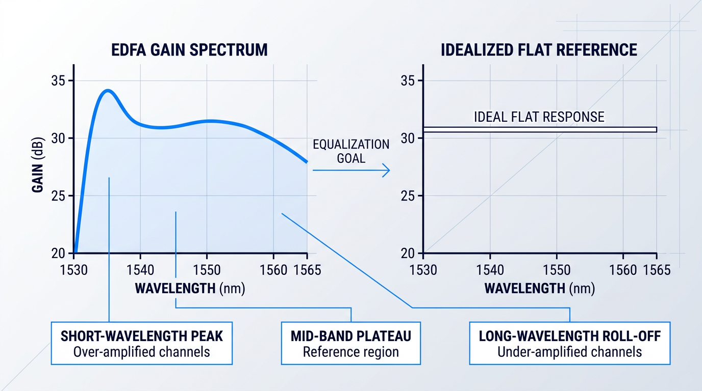
The result is a gain profile with a characteristic and unavoidable shape across the C-band: a pronounced gain peak at the shorter-wavelength edge of the band, a comparatively flatter plateau through the mid-band region, and a gradual roll-off toward the longer-wavelength edge.
Critically, this spectral shape is not static. As the amplifier's inversion level changes with input signal power or channel loading, the gain profile shifts — a phenomenon known as dynamic gain tilt. A highly inverted amplifier presents a different gain contour from a partially inverted one, meaning the non-uniformity problem varies with operating conditions, not just with amplifier design.
Consequences for WDM Systems
When many WDM channels traverse the same EDFA without equalization, channels near the short-wavelength gain peak are over-amplified while channels at lower-gain wavelengths are under-amplified. This produces channel power imbalance: some channels arrive at the receiver with far more optical power than others, making it impossible to simultaneously serve all channels within their required operating power range.
The consequences split in two directions. Under-amplified channels suffer degraded OSNR — they are weaker relative to the amplified spontaneous emission noise that accumulates at every stage. Over-amplified channels approach nonlinear thresholds in the transmission fibre, where Kerr effects and stimulated Raman scattering begin to corrupt the signal.
What makes this especially consequential for long-haul networks is the cascading effect. A single EDFA's gain ripple may appear small in isolation, but in a multi-span system with many in-line amplifiers, that per-stage ripple accumulates with each pass — channel power differentials that are modest after one span grow into system-limiting imbalances across a full long-haul or submarine chain.
Gain non-uniformity that seems negligible in a single EDFA becomes the dominant constraint on transmission reach when that ripple accumulates across tens or hundreds of in-line amplifiers — which is why gain equalization is a system necessity, not an optional refinement.
This is why gain equalization is treated as a system-level requirement in any serious multi-span WDM deployment. Two principal approaches address it: passive gain flattening filters (GFFs), which impose a fixed corrective attenuation profile, and dynamic gain equalizers (DGEs), which adapt to changing operating conditions. The sections that follow explore both, beginning with the passive filter technologies that form the backbone of most deployed systems.
Passive Gain Flattening Filters: Technologies and Trade-offs
Knowing that EDFA gain is wavelength-dependent is one thing; knowing how to correct it is another. The passive gain flattening filter (GFF) is the dominant engineering solution — a fixed optical element inserted into the amplifier that imposes a spectrally shaped loss to counteract the gain non-uniformity, leaving the composite response flat across the operating band.
The operating principle is the conceptual anchor for everything that follows: the GFF is designed with a transmission profile that is the inverse of the EDFA gain spectrum. Where the amplifier's gain is highest, the filter attenuates most; where gain is lowest, the filter transmits freely. The combined gain-plus-filter response satisfies the condition where the product of gain and filter transmission is constant across the band.
Before examining how different technologies achieve that inversion, it is worth establishing the metrics engineers use to specify and compare GFFs — these are the evaluation axes that give the technology survey below its practical meaning.
- Peak-to-peak error function (PPEF): Maximum deviation between the filter's actual transmission and its target profile across the operating band — the primary figure of merit for spectral matching accuracy.
- Modulation depth: The full attenuation range the filter can impose across its band; must be sufficient to correct the amplifier's gain non-uniformity, which can exceed 10 dB in practice.
- Insertion loss (excess loss): Loss beyond the intended attenuation profile. Every additional dB must be compensated by the amplifier, directly penalising power efficiency and noise figure.
- Polarisation-dependent loss (PDL): Variation in loss with polarisation state. PDL accumulates across cascaded components and introduces power uncertainty at the receiver; typically specified at 0.1 dB maximum.
- Polarisation mode dispersion (PMD): Differential group delay between polarisation states; significant for high-data-rate coherent channels. Typically specified at 0.1 ps maximum for GFF components.
- Return loss: Measures back-reflected power; high return loss (typically 50 dB or above) is critical for amplifier stability and preventing parasitic lasing.
- Operating wavelength range: The spectral window the filter covers; must encompass the full system band — C-band (1528–1565 nm), L-band (1570–1610 nm), or both.
With that vocabulary in place, the four principal filter technology families can be examined on their own terms — each with a distinct operating mechanism and a distinct set of strengths and limitations.
Thin-Film Dielectric Filters
Thin-film dielectric filters (TFFs) achieve spectral shaping through multilayer dielectric coatings deposited on a glass substrate: alternating layers of high- and low-refractive-index dielectric materials create wavelength-dependent constructive and destructive interference, producing a precisely engineered transmission profile.
TFFs are capable of very precise spectral matching. Industry data shows that PPEF below 0.1 dB is achievable for modulation depths up to approximately 6 dB, with PPEF below 0.4 dB for modulation depths of 8 dB or more; filters with modulation depths up to 16 dB have been demonstrated, though performance trade-offs become necessary at those extremes.
Excess insertion loss in TFFs is typically low, but there is a real trade-off: sharper spectral features in the target profile — steeper slopes, narrower notches — are harder to reproduce without increasing the layer count and, consequently, the excess loss.
The environmental credentials of hard-coated TFF designs are a genuine advantage for field-deployed systems. Modern ion-beam-sputtered dielectric coatings are robust to humidity, temperature cycling, and long-term ageing, and TFF technology benefits from decades of manufacturing maturity in the thin-film optics industry.
Long-Period Fibre Bragg Gratings
Long-period gratings (LPGs) operate on a fundamentally different principle from standard reflective FBGs. With grating periods typically in the range of hundreds of micrometres to a millimetre, LPGs couple light from the guided core mode into forward-propagating cladding modes at specific resonance wavelengths; because cladding modes are lossy, this coupling creates a broad transmission attenuation band at those wavelengths rather than a reflection.
The broad, smooth resonance of LPG coupling is well matched to the broad, smooth features of the EDFA gain spectrum — particularly the prominent peak around 1530 nm — making LPGs a natural fit for correcting the coarse gain shape.
That same smoothness is also a limitation: LPG resonances cannot easily reproduce gain profiles with sharp or complex spectral features, and their ability to achieve fine spectral sculpting is inherently constrained by the breadth of their attenuation bands.
LPGs exhibit significant temperature dependence in their resonance wavelengths — a liability for passive GFFs in variable-temperature environments, though this characteristic has been exploited in compound GFF designs where a conventional filter and an LPG are combined to compensate for EDFA gain temperature dependence (discussed further in the section on environmental stability). The all-fibre construction of LPG-based GFFs confers inherently low insertion loss and low PDL.
Tilted Fibre Bragg Gratings
Tilted fibre Bragg gratings (TFBGs) have their grating planes written at an angle to the fibre axis rather than perpendicular to it. This tilt couples light from the core mode to radiation modes or cladding modes rather than reflecting it back, creating spectrally selective attenuation — the mechanism that makes them useful as gain flattening elements.
By controlling the tilt angle, grating period, and apodisation profile, TFBGs can be designed to produce complex, arbitrary attenuation spectra — making them potentially more flexible than LPGs for matching intricate gain profiles with sharper spectral features.
Two practical limitations constrain TFBG performance. First, the asymmetry introduced by the tilt can produce polarisation-dependent loss, which must be carefully managed in long-haul systems where PDL accumulates across many components. Second, manufacturing imperfections in the grating profile can introduce unwanted spectral ripple in the transmission spectrum, affecting the achievable PPEF.
Waveguide-Based Approaches
Planar lightwave circuit (PLC) approaches implement spectral shaping using integrated optical waveguide structures — typically Mach-Zehnder interferometer (MZI) lattices or other interferometric arrangements — fabricated on a planar substrate, most commonly silica-on-silicon.
The MZI operating principle relies on splitting an input signal into two arms of differing optical path lengths, then recombining them: the resulting interference is constructive or destructive depending on wavelength, producing a periodic transmission spectrum whose free spectral range is set by the path-length difference. Cascaded MZI stages can synthesise more complex spectral shapes.
The integration potential is a genuine architectural advantage: waveguide-based GFFs can in principle combine filtering, splitting, and combining functions on a single chip, which is attractive for compact amplifier module designs.
The principal challenge for waveguide-based GFFs is the thermo-optic effect: the refractive index of silica waveguides varies with temperature at approximately 10⁻⁵ per °C, causing the interferometric spectral profile to shift with ambient temperature. For a passive GFF with a fixed target profile, this is a significant liability in field-deployed systems operating across a wide temperature range.
Athermalization strategies — packaging with materials of opposing thermal expansion, active temperature control, or design-level index compensation — can mitigate this effect, but each approach adds cost and complexity that must be weighed against the integration benefits.
Taken together, the four technology families cover a wide range of operating principles and performance envelopes. The table below compares them across the key evaluation axes that drive practical filter selection.
| Technology | Spectral Complexity / PPEF | Insertion Loss (Excess) | PDL | Temperature Stability | Manufacturing Maturity |
|---|---|---|---|---|---|
| Thin-film dielectric filter (TFF) | High — PPEF <0.1 dB at up to 6 dB modulation depth; <0.4 dB at 8 dB+; up to 16 dB depth demonstrated | Low to Medium — varies with profile complexity; steep profiles increase layer count and loss | Low — typically 0.1 dB max | High — hard-coated designs robust to humidity and temperature cycling | High — decades of thin-film manufacturing infrastructure |
| Long-period grating (LPG) | Medium — smooth, broad attenuation bands suit coarse EDFA gain shape; limited fine spectral sculpting | Low — 0.5–1.5 dB typical; all-fibre construction minimises coupling loss | Low — inherently low due to all-fibre symmetric construction | Low — significant resonance wavelength shift with temperature | Medium — established but more specialised than TFF |
| Tilted fibre Bragg grating (TFBG) | Medium-High — arbitrary attenuation spectra possible via tilt angle and apodisation control; spectral ripple is a practical limit | Low-Medium — 1–3 dB typical; grating imperfections contribute additional loss | Medium — tilt asymmetry introduces PDL that requires careful management | Medium — FBG Bragg wavelength shifts ~10 pm/°C; compensation packaging available | Medium — established FBG fabrication base; tilted variant more specialised |
| Waveguide / PLC (MZI lattice) | High — complex spectral shapes achievable via cascaded interferometer stages | Medium — fibre-to-chip coupling loss adds to waveguide propagation loss | Low — symmetric waveguide structures have inherently low PDL | Low — thermo-optic coefficient ~10⁻⁵/°C causes profile shift; athermalization required | Low-Medium — PLC fabrication mature in telecom, but GFF-specific designs less widespread |
Comparison of GFF technology families across key engineering evaluation axes to support filter selection decisions.
The table makes clear that no single technology dominates across all axes. TFFs offer the most mature combination of precise spectral shaping, low excess loss, and environmental stability — which explains their dominant position in deployed WDM systems. LPG-based filters are well suited to applications where the gain profile is smooth and insertion loss budget is tight, but their temperature sensitivity demands careful management. TFBGs offer more spectral flexibility than LPGs but introduce PDL and ripple trade-offs that must be evaluated against system requirements. Waveguide-based approaches are compelling where integration density matters, but the thermo-optic challenge makes them less straightforward to deploy passively in variable-temperature environments without additional engineering.
The practical selection logic follows from the gain profile's spectral character: a smooth, broad correction favours LPGs; a complex profile with steep features and demanding PPEF requirements favours TFFs or TFBGs; and where chip-level integration is the priority, waveguide approaches merit serious consideration alongside their thermal management requirements.
The EDFA gain spectrum depends on erbium fibre composition, pump wavelength and power, signal loading, and operating inversion level. No two amplifier designs produce exactly the same profile, which means a GFF designed for a generic C-band EDFA will rarely match a specific system with the precision that high-performance WDM applications require. Custom filter design — matched to the amplifier's measured gain data — is the norm, not the exception.
This customisation imperative applies regardless of which filter technology is selected. The gain profile is a measured input, not an assumption, and the filter manufacturer designs to match it — selecting the right technology family narrows the design space, but achieving the required PPEF in a specific amplifier context requires a filter tailored to that amplifier's actual spectral characteristics.
With the technology families and their trade-offs understood, the next engineering decision is where in the amplifier chain the GFF is placed — and that choice carries real consequences for noise figure and power efficiency.
GFF Placement: Noise Figure and Efficiency Trade-offs
Once you have selected a gain flattening filter, the next question is deceptively simple: where in the amplifier chain does it go? The answer matters far more than it might appear, because the GFF's insertion loss does not have a fixed cost — its impact on noise figure and pump power efficiency shifts dramatically depending on whether that loss falls before, within, or after the gain medium.
The difficulty is that noise figure and power efficiency pull in opposite directions across the three viable positions: input, output, and mid-stage insertion in a dual-stage EDFA. Optimising for one tends to penalise the other, and the resolution of that tension carries its own architectural cost.
The Three Placement Options and Their Physics
Output-stage placement is the most noise-benign of the three positions. By the time the signal reaches a filter at the amplifier's output, it has already been fully amplified — it sits well above the quantum noise floor, so the filter's attenuation does not meaningfully degrade the amplifier's noise figure.
The power efficiency penalty, however, is real. The amplifier must generate more output than the system actually needs, only for the GFF to absorb the excess. Pump energy is consumed producing signal power that is immediately discarded — an inefficiency that becomes increasingly costly at high output powers.
Input-stage placement reverses this trade-off entirely. Attenuating a weak signal before it enters the gain medium is the worst possible position for noise figure. The physics here follow the Friis cascade noise principle: any passive loss element placed ahead of the first stage of gain adds its loss directly to the system noise figure, with no preceding gain to suppress the contribution.
A signal that enters the amplifier already weakened forces the gain medium to work from a lower starting point, and the spontaneous emission noise generated in the first pass of amplification dominates the output. The power efficiency argument runs the other way — a weaker input extracts less power from the inversion, so the pump is utilised more efficiently — but in practice, no noise-sensitive telecom application accepts the noise figure cost that input placement imposes.
Mid-stage insertion, within a dual-stage EDFA architecture, is the engineering compromise that the industry has settled on for noise-critical applications. The first amplifier stage raises the signal to a level where mid-stage loss is no longer catastrophic from a noise perspective: the gain of the first stage substantially suppresses the noise contribution of the filter, in the same way that Friis cascade analysis shows that high-gain first stages reduce the noise impact of subsequent lossy elements.
The second stage then amplifies the filtered signal to the required output power. The result is a system that avoids the full noise penalty of input placement and the full power waste of output placement — though it does not fully escape either.
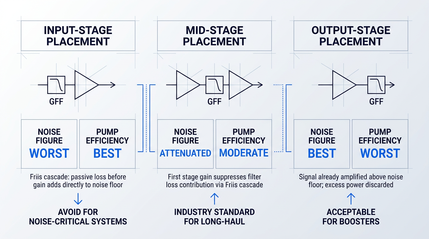
The noise figure penalty from mid-stage loss is real but substantially attenuated by the first stage's gain. If the first stage delivers, say, 10–15 dB of gain before the filter, the filter's insertion loss contribution to the overall system noise figure is divided down by that gain factor — meaning several dB of mid-stage insertion loss translates to a much smaller noise figure degradation at the system level than the same loss placed at the input.
The precise magnitude depends on the first-stage gain and the filter's insertion loss in each spectral band, but the directional principle is robust: more first-stage gain means less noise figure sensitivity to mid-stage loss, which is why dual-stage amplifier designs often optimise the first stage for gain rather than output power.
Mid-stage insertion is not, however, a free upgrade. It requires a dual-stage amplifier architecture with a physically accessible mid-stage port — an interface between the two gain stages where the signal can be extracted, passed through the filter, and re-injected. This demands additional fibre couplers, isolators, and connectors at the mid-stage interface, each of which introduces its own coupling loss.
The component count increase is non-trivial, and the additional splices and connectors at the mid-stage interface add to both insertion loss and the potential for reflections that can destabilise the amplifier. Design and manufacturing complexity rises accordingly. For high-volume deployments, this translates directly into cost and yield considerations that a simple single-stage amplifier with an output-placed filter does not face.
Matching Placement to Amplifier Type
- Long-haul in-line amplifiers: Mid-stage insertion is the standard approach. Noise accumulates linearly across cascaded amplifier spans, so each amplifier's noise figure directly affects end-to-end system reach.
- Booster amplifiers: Output-stage placement is often acceptable. The input signal is already strong, and maximising launch power matters more than minimising the noise figure increment.
The distinction maps cleanly onto system priorities. In a long-haul network with dozens of in-line amplifier spans, even a fraction of a dB of excess noise figure per amplifier compounds across the chain — the aggregate impact on optical signal-to-noise ratio at the receiver can be severe. Mid-stage insertion, despite its architectural overhead, is the only placement that keeps per-amplifier noise figure within budget.
For a booster amplifier sitting immediately after a transmitter, the calculus is different. The signal entering the booster is already well above the noise floor, and the amplifier's own noise figure contributes relatively little to the end-to-end OSNR. Output-stage placement is simpler, cheaper, and entirely adequate — the noise figure premium of mid-stage insertion buys little in this context.
Choosing mid-stage GFF placement in a dual-stage EDFA is the right answer for noise-sensitive in-line amplifiers — but it is a genuine design commitment that adds component count, coupling losses, and manufacturing complexity. The noise figure benefit is real; so is the cost.
With the placement question resolved, the next practical challenge is ensuring the filter actually delivers its designed spectral correction once it is installed in a real system — where ambient temperature varies, and where the filter's transmission profile can drift in ways that reintroduce the channel power imbalance it was designed to eliminate.
Temperature Stability of Gain Flattening Filters
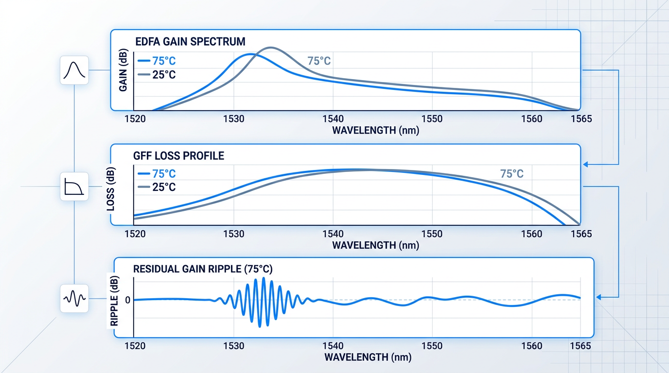
A gain flattening filter is designed at a reference temperature — typically 25°C on a lab bench — to complement the EDFA gain spectrum it will correct. The engineering challenge that most guides overlook is this: both the filter's loss profile and the EDFA's gain spectrum change with temperature, but they change in fundamentally different ways, so their errors do not cancel. The result is a residual gain ripple that grows as the deployment temperature departs from the design point.
A thin-film GFF typically responds to temperature by shifting its spectral features to longer or shorter wavelengths — the entire loss profile slides along the wavelength axis. The EDFA gain spectrum, by contrast, changes shape: the peak in the 1530–1535 nm region grows or shrinks relative to the rest of the C-band rather than shifting uniformly. Because these two responses are mismatched in character, the equalization that was accurate at the design temperature degrades as temperature changes — and it degrades in a way that cannot be corrected simply by recentring the filter.
Temperature Sensitivity of Thin-Film Dielectric Filters
The physical mechanism behind thin-film filter drift is well established: the thermo-optic effect causes the refractive indices of the coating layers to change with temperature, while thermal expansion simultaneously alters the physical thickness of each layer.
Together, these two effects shift the filter's spectral features along the wavelength axis. According to Iridian's wavelength budgeting data, the temperature coefficient of a thin-film filter typically ranges from 1–2 pm/°C to 10–20 pm/°C, depending on the substrate and coating materials used.
The practical consequence becomes clear with a concrete example: a filter with a 10 pm/°C coefficient operating across a 100°C temperature range accumulates approximately 1 nm of spectral drift between its thermal extremes.
One nanometre of drift is not negligible anywhere in the C-band, but it is most damaging in the 1530–1535 nm region, where the EDFA gain slope is steepest and the gain is most sensitive to small wavelength errors — making this the primary zone of concern for system engineers evaluating temperature performance.
Coating process also matters significantly. Ion-beam sputtered (IBS) coatings are substantially denser than thermally evaporated soft coatings, exhibiting negligible spectral drift and excellent environmental stability; ion-assisted deposition (IAD) offers an intermediate improvement over standard e-beam evaporation.
Commercial GFFs from established suppliers are qualified to defined operating temperature ranges — Lumentum's thin-film GFF, for example, specifies an operating temperature range of 0 to 70°C and is qualified to Telcordia GR-1221 requirements, giving buyers a traceable performance envelope rather than a single 25°C datasheet value.
Long-Period Gratings and the Compound GFF Approach
Long-period fibre gratings (LPGs) exhibit substantially larger wavelength-shift temperature dependence than thin-film filters. Peer-reviewed measurements place LPG temperature sensitivities in the range of approximately 0.32 nm/°C for standard silica LPGs, rising to 0.56–0.60 nm/°C for uncoated LPGs in water, and 0.86 nm/°C for polymer-recoated variants — orders of magnitude larger than the ~10 pm/°C baseline of a standard FBG.
Used in isolation as a passive GFF, this large temperature coefficient is a liability: the filter's spectral shape drifts substantially across a realistic deployment temperature range, undermining gain flatness.
Furukawa Electric's research identified a way to turn this liability into an asset — the compound GFF approach, which combines a conventional GFF (small temperature coefficient, stable spectral shape) with a long-period grating (large temperature coefficient) to produce a composite filter whose temperature response partially corrects for the EDFA gain spectrum's own temperature-induced shape change.
The mechanism relies on the fact that the EDFA gain spectrum's temperature sensitivity is concentrated below 1535 nm, and that a filter with a negative temperature coefficient in that region — provided by the LPG acting as a reverse-slope filter — can partially counteract the gain change that would otherwise occur there.
Furukawa's prototype results demonstrate the approach's effectiveness: in a 13 dB gain EDFA fitted with the compound GFF, gain variation across the 0–65°C temperature range was reduced from 0.79 dB to 0.25 dB, with gain flatness maintained below 0.60 dB at all temperatures across that range.
This is not a theoretical curiosity — Furukawa released the compound gain equaliser as a product, with a 26 dB gain EDFA variant achieving a total gain temperature variation of just 0.45 dB across 0–65°C. The approach requires careful co-design of the two filter elements, with the LPG's period and fibre composition chosen to produce the specific temperature coefficient needed to complement the conventional GFF.
Thin-Film Filter Design Strategies for Thermal Stability
Beyond the compound GFF approach, there are several filter-level design strategies that reduce the intrinsic temperature drift of thin-film GFFs.
- Low-expansion substrates: Substrate materials with low coefficients of thermal expansion reduce the physical thickness change component of spectral drift, lowering the overall temperature coefficient.
- Hard-coating processes: IBS and IAD coatings are denser and less porous than soft e-beam coatings, reducing both humidity sensitivity and thermally induced spectral shift.
- Athermal packaging: Mounting the filter in a housing engineered to mechanically compensate for thermal expansion can reduce net spectral drift without changing the coating itself.
- Temperature-characterised datasheets: Some designs document worst-case error function degradation across a specified operating range — buyers should request this data, not assume 25°C performance holds in the field.
The practical implication for procurement is straightforward: a filter's ambient-temperature performance specification is a necessary condition, not a sufficient one, for field deployment.
Practical Implications for System Engineers
Field-deployed amplifiers — outside-plant nodes, amplifiers in industrial or defence environments, and submarine repeaters — routinely experience temperature swings that a 25°C lab measurement does not capture.
The gain flatness budget must account for temperature-induced filter drift. A GFF specified at ±0.3 dB peak-to-peak error function (PPEF) at 25°C that drifts by an additional ±0.2 dB across its operating temperature range contributes an effective per-amplifier ripple of ±0.5 dB — not the ±0.3 dB figure on the datasheet.
In a long-haul WDM system with many in-line amplifiers, per-amplifier filter drift does not average out — it accumulates. A small temperature-induced ripple error that looks manageable at a single amplifier becomes a large channel power differential at system scale, consuming margin that cannot be recovered without active equalization.
The submarine case illustrates the extreme end of this problem. As noted in ITU-T guidance on repeatered submarine systems, gain flatness requirements are extremely tight in transoceanic links where the number of amplifiers can reach several hundred — because impairments due to non-flatness of the cumulative gain curve accumulate across the entire chain.
For this reason, submarine-grade GFFs must satisfy qualification criteria for filter shape stability under both temperature fluctuations and long-term ageing — a level of environmental testing that terrestrial filters may not undergo, and that is documented in standards such as Telcordia GR-1221.
The temperature sensitivity characteristics of the principal GFF technologies differ by orders of magnitude across technology families, with direct consequences for how much of the gain flatness budget temperature drift consumes in a given deployment.
| Filter Technology | Typical Temperature Coefficient | Primary Thermal Mechanism | Stability Characteristic |
|---|---|---|---|
| Thin-film dielectric (soft coating / e-beam) | ~10–20 pm/°C | Thermo-optic effect + thermal expansion; porous layers absorb moisture | Lower stability; spectral shift worsened by humidity exposure |
| Thin-film dielectric (hard coating / IBS or IAD) | ~1–2 pm/°C (lower end of Iridian range) | Thermo-optic effect + thermal expansion; dense layers resist moisture | Higher stability; negligible spectral shift; preferred for field deployment |
| Fibre Bragg grating (FBG) | ~10 pm/°C at 1550 nm | Thermo-optic effect + thermal expansion of silica grating period | Stable and predictable; well-characterised baseline for compensation |
| Long-period fibre grating (LPG) — standard silica | ~320 pm/°C (0.32 nm/°C) | Differential thermo-optic effect between core and cladding modes | High drift in isolation; exploited in compound GFF approach |
| Long-period fibre grating (LPG) — polymer-recoated | ~860 pm/°C (0.86 nm/°C) | Enhanced by polymer coating thermo-optic contribution | Highest drift; useful only in controlled compound GFF co-design |
Comparison of temperature sensitivity across GFF filter technologies using sourced figures, to help engineers evaluate thermal stability trade-offs in technology selection.
The contrast between LPG and hard-coated thin-film coefficients spans roughly two orders of magnitude — the polymer-recoated LPG drifts at 0.86 nm/°C against a hard-coated thin-film filter's ~1–2 pm/°C. For a passive GFF used alone, this makes LPGs a poor choice in thermally challenging environments. The compound GFF approach reframes the LPG's large coefficient as an asset, but only when it is deliberately co-designed with a conventional filter element to exploit that drift in a controlled direction.
For engineers specifying filters for demanding deployments, the actionable guidance is consistent across all technology families: request temperature-characterised performance data covering the full operating temperature range of the installation, not just the ambient-temperature specification.
Where temperature-induced gain variation exceeds what passive filter design strategies can manage — particularly in systems with rapidly changing operating conditions or very tight per-amplifier budgets — dynamic gain equalizers offer an active solution that can track and correct the gain profile in real time, as the next section explores.
Dynamic Gain Equalizers: When Static Filters Fall Short
A passive gain flattening filter is designed for a specific operating point — a fixed gain level, a fixed channel loading, a fixed temperature. The world that a deployed amplifier actually inhabits rarely stays fixed.
When channel loading changes due to add/drop events, the amplifier's saturation level shifts and the gain spectrum shape changes with it. When Raman-induced tilt accumulates differently across varying traffic loads, or when amplifiers age and their gain profiles drift beyond the GFF's original design point, the passive filter is now correcting the wrong curve. This is not a failure of the GFF — it is a fundamental mismatch between a static correction and a dynamic problem.
The scale of the consequence is what motivates a different class of device. Identical amplifiers built to the same design carry identical residual gain shapes, so their errors add linearly down a cascade rather than averaging out. A 0.35 dB per-span residual ripple — unremarkable on a single amplifier — reaches 4.2 dB after twelve spans, and 4.2 dB of differential spread across the channel comb represents the entire OSNR margin separating DP-16QAM from DP-QPSK.
This arithmetic defines the threshold, not a universal prescription. Short-haul or lightly cascaded systems with stable channel loading and well-matched GFFs do not need dynamic correction. The scenarios that genuinely warrant it are more specific.
- Reconfigurable WDM networks: Significant channel add/drop activity shifts amplifier saturation continuously, making any fixed GFF profile an approximation at best.
- Ultra-long-haul systems: Accumulated gain tilt across many spans exceeds the passive filter's correction range, requiring active trimming at intervals along the chain.
- C+L band systems: Raman-induced inter-band tilt varies with traffic load and cannot be fully pre-compensated by a static filter profile.
- Ageing amplifier plants: Gain profiles drift over years of operation beyond what the original GFF was designed to handle, including temperature-driven spectral shifts.
A dynamic gain equalizer (DGE) addresses these scenarios by functioning as a wavelength-dependent optical attenuator whose loss-versus-frequency profile can be commanded in real time while traffic runs.
The typical closed-loop architecture pairs the DGE with an optical channel monitor (OCM) that measures the per-channel power spectrum continuously. A controller computes the required per-wavelength attenuation corrections and commands the DGE to apply them, driving the output spectrum toward a flat target profile. The loop runs continuously, updating as operating conditions change.
DGE Technology Families
Three principal technology families implement the DGE function, each with a distinct operating mechanism and a different set of practical trade-offs.
MEMS-Based Dynamic Gain Equalizers
MEMS-based DGEs use a free-space grating spectrometer to spatially disperse the WDM signal so that each spectral channel illuminates a separate micromirror in a linear array. Tilting each mirror varies the coupling efficiency back into the output fibre, producing a wavelength-dependent attenuation profile that can be updated by adjusting mirror angles under electronic control.
The practical characteristics are well established. MEMS DGEs require no temperature control, offer fast response, and cover the full C-band from 1528 nm to 1570 nm. Peer-reviewed characterisation of MEMS spectral equalizers reports 40–80 channel capacity with 6–7 dB insertion loss and 20–30 dB dynamic range. One commercially documented MEMS DGE specifies insertion loss below 6 dB, PDL below 0.25 dB, residual ripple below 0.30 dB, and maximum attenuation of 15 dB — figures consistent with the broader literature.
Liquid Crystal and LCoS-Based DGEs
Liquid crystal DGEs control attenuation by exploiting the voltage-dependent birefringence of liquid crystal cells: applying a voltage rotates the polarisation state of the incident light, and a subsequent polariser converts that polarisation change into a controllable amplitude loss. In a multi-cell arrangement, different cells address different spectral bands, producing a programmable attenuation profile across the WDM comb.
Liquid crystal on silicon (LCoS) technology — familiar from wavelength-selective switches (WSS) in ROADM architectures — has been adapted for inline gain equalisation. An LCoS device places a high-resolution pixel array on a CMOS silicon backplane, allowing each pixel to impose an independently controlled phase or amplitude response on a spatially dispersed wavelength band. This achieves spectral resolution approaching individual channel spacing, enabling per-channel power control within a single module. The same LCoS engine that performs ROADM switching can therefore also serve as a dynamic gain equalizer without a separate component, a convergence that is driving integrated C+L band DGE modules.
Acousto-Optic Tunable Filters as DGEs
The all-fibre acousto-optic tunable filter (AOTF) operates on a fundamentally different principle: an acoustic transducer drives a continuous-wave acoustic signal along a section of single-mode fibre, creating a long-period grating-like structure that couples a narrow band of light from the guided core mode into lossy cladding modes. The coupled light cannot return to the core and is stripped away, producing a tunable notch in the transmission spectrum.
Two parameters are independently controllable: the RF frequency sets the centre wavelength of the notch, and the drive voltage sets the notch depth. This independence gives the AOTF considerable flexibility in tailoring filter shapes. Multiple notches are achieved either by cascading several AOTF stages in series or by applying multiple RF frequencies simultaneously to a single transducer — each frequency creates its own independent notch.
The defining practical advantage of the AOTF is very low insertion loss per stage, since attenuation occurs directly in the fibre without demultiplexing or free-space coupling. Cascading additional stages to achieve greater spectral resolution adds only the incremental loss of the fibre splices between them. Response time is approximately 40 microseconds — roughly 10 to 100 times faster than comparable technologies at the time the all-fibre AOTF was characterised — which becomes relevant in agile networks where optical switches create rapid channel loading changes.
Two Architectural Approaches to Equalisation
Across all three technology families, DGEs implement one of two fundamental filter architectures, and the choice between them carries real system implications.
A channel-by-channel equalizer demultiplexes the WDM signal into individual channels, attenuates each independently, then remultiplexes. This offers high spectral resolution and fine-grained per-channel control, making it well suited to correcting sharp features in the gain spectrum. The trade-off is that the device is tied to a specific channel plan — it must be configured for a predetermined wavelength grid and channel spacing — and the demultiplexer/multiplexer pair can introduce passband narrowing and additional spectral dispersion, creating a power penalty in long chains of such devices.
A continuous envelope equalizer shapes the spectral envelope without demultiplexing, applying a smooth, continuous attenuation function across the band. Because it never resolves individual channels, it is independent of the channel plan and introduces no passband narrowing — characteristics that make it well suited for inline amplifier applications where the gain profile from an EDFA is itself a smoothly varying curve. The limitation is lower spectral resolution: sharp features in the gain spectrum that require correction at sub-nanometre scales may not be fully addressed.
Neither architecture is superior in the abstract. Channel-by-channel designs suit systems that need fine per-channel power trimming or wavelength blocking; continuous envelope designs suit systems that need transparent, channel-plan-independent gain shape correction across a long amplifier cascade.
Every DGE adds insertion loss — typically 3–7 dB — which carries a direct noise figure cost. Mid-stage placement inside a dual-stage EDFA, with adequate first-stage gain, is the standard mitigation. A DGE's value is measured by whether the OSNR recovered by correcting residual ripple exceeds the OSNR cost of its own insertion loss.
When specifying a DGE, system engineers evaluate across several axes. Equalization depth (dynamic range) defines how large a per-channel attenuation the device can apply; typical figures run 10–20 dB. Residual ripple after closed-loop correction should reach approximately ±0.25–0.3 dB for ultra-long-haul applications. Insertion loss of 3–7 dB is the norm, with the noise figure penalty managed through mid-stage placement as established in the filter placement discussion earlier in this guide. PDL should be held below 0.3 dB to avoid creating a polarisation-dependent power variation that amplifier gain cannot correct. Spectral resolution determines whether the device can address narrow gain features or only broad envelope shapes. Response speed matters most in agile networks where channel loading changes rapidly.
The deployment economics reinforce the principle that DGEs are not a replacement for passive GFFs. At a cost of roughly $10,000–$12,000 per unit, DGEs are placed at intervals of every four to five amplifiers — positioned where accumulated residual ripple has grown to the point where correction is necessary, not at every span.
When a DGE is deployed, mid-stage placement inside a dual-stage EDFA remains the preferred position, for the same reason it is preferred for passive GFFs: adequate first-stage gain suppresses the noise figure contribution of the DGE's insertion loss to a fraction of a decibel. A practical amplifier design therefore uses a passive GFF to handle the bulk of the static gain correction, with the DGE providing dynamic trimming on top — the GFF reduces the correction range the DGE must accommodate, and the DGE handles what the GFF cannot.
With the technology families and their trade-offs understood, the practical question becomes how to specify the right equalization approach for a given system — which is where the next section picks up.
Design Considerations for WDM System Engineers
Understanding how a gain flattening filter works is not the same as knowing how to specify one. The gap between those two things — between technology literacy and engineering specification — is where real systems encounter problems that no amount of post-deployment tuning can fully correct.
The parameters that define a GFF requirement are interconnected: you cannot fix an insertion loss budget without knowing your placement decision, you cannot set a target peak-to-peak error function (PPEF) without knowing your residual ripple allocation, and you cannot specify bandwidth without knowing your band plan. What follows is a decision framework that treats those axes as a system, not a checklist.
Bandwidth Coverage: C-Band, L-Band, or C+L
The first axis is also the most fundamental: the filter must cover the full operating wavelength range of the system. But bandwidth coverage is not simply a matter of stating a wavelength range — it is a gain-profile question.
The C-band (approximately 1530–1565 nm) and the L-band (approximately 1565–1625 nm) present meaningfully different gain shapes. As covered in the Background section, erbium's gain spectrum is strongly inversion-dependent: high inversion produces a pronounced peak near 1530 nm, while lower inversion shifts the gain maximum toward longer wavelengths. L-band EDFAs run at lower average inversion and require longer erbium-doped fibre to achieve comparable gain — and the resulting gain profile has a different shape and magnitude from its C-band counterpart.
A GFF designed for C-band operation cannot be repurposed for L-band use. The correction profile is specific to the gain shape it was designed to invert, and those shapes are not interchangeable.
A C+L combined system compounds the challenge further. Inter-channel stimulated Raman scattering transfers power from C-band channels to L-band channels across every span, introducing a spectral tilt that scales with both total power and total bandwidth. The gain equalisation strategy for a C+L system must account for this dynamic power transfer, not just the static erbium gain profile in each band.
Insertion Loss Budget: Every Decibel Has a Cost
Every decibel of GFF insertion loss must be recovered somewhere in the link budget — through additional amplifier gain, which costs pump power and degrades noise figure. Excess insertion loss (loss beyond the intended attenuation profile) is not a passive inconvenience; it is a direct tax on system OSNR.
This is why minimising excess loss is a primary filter selection criterion, not a secondary nicety. The insertion loss budget and the placement decision are coupled: as discussed in the placement section, locating the GFF at mid-stage of a dual-stage amplifier allows the first gain stage to suppress the noise contribution of the filter's loss. But that mid-stage loss budget is not unlimited — the amplifier design sets a ceiling, and the GFF must fit within it.
Practically, thin-film GFFs for C-band and L-band applications can achieve insertion loss below 0.2 dB. Excess loss beyond the intended attenuation profile should be treated as a hard specification constraint, not a soft preference, when engaging a filter supplier.
Gain Profile Measurement: The Upstream Constraint
A filter manufacturer needs accurate gain data from the specific amplifier design — measured at the intended operating point — to produce a matched GFF. The operating point means the actual gain level, signal loading, and temperature at which the amplifier will run in the deployed system, not a convenient laboratory condition.
What many engineers underestimate is that the quality of the gain profile measurement directly limits the achievable PPEF. A filter manufacturer can only correct what they can see in the data provided. If the gain spectrum is measured at the wrong loading, the wrong gain setpoint, or the wrong temperature, the GFF will be designed to invert the wrong curve — and no amount of manufacturing precision can compensate for that upstream error.
The achievable peak-to-peak error function is bounded by the accuracy of the amplifier gain spectrum the buyer provides. A poorly characterised gain profile means the GFF cannot be designed to match it accurately, regardless of the filter manufacturer's capability. Measure at the intended operating point — the right gain level, signal loading, and temperature — before engaging a supplier.
When preparing a GFF specification, a supplier will typically require: the measured gain spectrum at the intended operating point, the operating wavelength range, the target PPEF, and the insertion loss and polarisation-dependent loss (PDL) constraints. The smoothness and slope of the target gain curve also influence the minimum achievable PPEF — steeper or more complex gain shapes impose tighter demands on the filter design.
Residual Ripple Budget in a Cascaded Chain
Specifying a GFF for a single amplifier is a component problem. Specifying it for a long-haul system with dozens of in-line amplifiers is a system problem — and the distinction changes the target.
As established in the Background section, residual gain ripple accumulates across a cascaded amplifier chain. When every amplifier in the chain carries the same GFF design with the same error function, the residual errors add coherently — linearly with span count, not as the square root. A per-amplifier residual of ±0.5 dB becomes a 10 dB accumulated spread after 20 spans if left uncorrected.
The practical implication is that the residual ripple budget for each amplifier is set by dividing the total allowable channel power differential at the system receiver across all amplifiers in the chain. For terrestrial long-haul systems, a residual ripple of ±0.5 dB per span is a common design target; undersea systems require considerably tighter values — systematic gain equalisation errors must be held within approximately 50 mdB per amplifier to prevent unacceptable channel power differentials over a chain of 120 or more amplifiers.
Tighter per-amplifier targets require either a better PPEF from the passive GFF, or more frequent dynamic correction points using a DGE. Where the passive filter's achievable PPEF cannot meet the per-amplifier budget, a DGE is not a luxury — it is the required engineering response.
| System Type | Per-Amplifier Residual Ripple Target | End-of-System Channel Power Flatness Target |
|---|---|---|
| Terrestrial long-haul | ±0.5 dB per span | ±1 dB at receive terminal |
| Undersea (120+ amplifiers) | ~50 mdB per amplifier | Tighter — set by system margin allocation |
| Extended-reach (20 spans) | Residual ripple below ±0.25 dB required | Accumulated error function limits transmission distance |
Comparison of residual ripple and channel flatness targets by system type, grounded in published figures from MapYourTech and Lightwave Online sources.
The table makes the stakes concrete: the per-amplifier target for an undersea system is an order of magnitude tighter than for a terrestrial link. Specifying the same GFF PPEF across both application types without adjusting for cascade length is a common design error — one that the link budget will eventually expose.
Secondary Axes: PDL, PMD, Spectral Resolution, and System Integration
Four additional parameters complete the specification framework. They are less dominant than insertion loss, gain measurement quality, and ripple budget, but omitting any of them from a demanding application produces a specification that will fail in the field.
- Polarisation-Dependent Loss (PDL): PDL accumulates stochastically across components and creates unpredictable power variation at the receiver. Values below 0.3 dB are required for long-haul applications; FBG-based filters exhibit inherently lower PDL than thin-film designs.
- Polarisation Mode Dispersion (PMD): A secondary concern that grows in importance at higher channel data rates. Different filter technologies contribute differently to PMD; specify it explicitly for 400G and above applications.
- Spectral Resolution: Dense WDM systems at 50 GHz or 100 GHz channel spacing impose tighter resolution requirements. A filter adequate at 200 GHz spacing may introduce passband narrowing or inter-channel crosstalk at 50 GHz.
- System Element Interaction: DCMs, ROADMs, and transmission fibre all introduce wavelength-dependent loss. The GFF target correction profile must account for the full amplifier module's passive component losses, not just the EDF gain shape in isolation.
On PDL: the Lightwave Online DGE evaluation literature places the acceptable threshold at values below 0.3 dB for long-haul applications, with tighter targets appropriate for ultra-long-haul and undersea deployments. As noted in the filter technology section, FBG-based filters achieve very low PDL by virtue of operating entirely within the fibre core — a genuine technology differentiator in PDL-sensitive applications.
On system element interaction: the ScienceDirect GFF literature is explicit that the GFF design must account for the wavelength-dependent loss of all passive components within the amplifier module. A GFF specified against the bare EDF gain profile, without folding in the loss contributions of WDM couplers, isolators, and any mid-stage elements, will produce a residual error function that no amount of PPEF optimisation can correct.
With these parameters defined — bandwidth, insertion loss budget, gain profile measurement quality, residual ripple allocation, PDL, PMD, spectral resolution, and system element interaction — the specification is ready for a supplier conversation. The next section addresses what that collaboration entails and what to expect from the custom filter development process.
Sourcing a GFF: What to Expect from a Supplier
Engineers who approach GFF procurement as a catalogue exercise — browsing standard part numbers until something looks close enough — consistently run into the same problem: there is no close enough.
An EDFA's gain spectrum is shaped by erbium fibre composition, pump power, amplifier architecture, signal loading, and operating point, and these variables combine differently in every design. The gain profile that results is essentially unique to that system, which means the filter that corrects it must be designed against that system's measured data — not against a generic approximation.
The practical implication is that custom filter design is the default engagement model, not a premium option. Coming to a supplier with accurate, well-conditioned measurements is what makes a productive collaboration possible.
What to Bring to a GFF Supplier
The quality of the filter design is bounded by the quality of the input data. A supplier can only design to what they are given, and a gain measurement taken at the wrong operating point or with insufficient signal-to-noise will produce a filter that cannot meet specification — regardless of how capable the supplier is.
- Measured gain spectrum: Taken at the intended operating point: target gain level, actual signal loading, and operating temperature. This is the foundational input; everything else is secondary.
- Wavelength range: C-band, L-band, or a combined C+L requirement. Defines the spectral extent the filter must cover and constrains technology selection.
- Target PPEF: The peak-to-peak error function budget the system can tolerate. Tighter targets demand more precise gain data and more design iterations.
- PDL and PMD limits: Hard constraints on polarisation-dependent loss and polarisation mode dispersion. Both accumulate across cascaded spans and must be specified upfront.
- Insertion loss budget: The maximum excess insertion loss the amplifier design can absorb without compromising noise figure or output power targets.
One point deserves particular emphasis: the gain measurement must be taken at the amplifier's actual intended operating point, not at a convenient bench condition. A measurement captured at the wrong gain level or with partial channel loading will produce a filter optimised for a state the deployed amplifier never inhabits.
Evaluating a GFF Supplier's Genuine Capability
Not all GFF suppliers occupy the same position in the supply chain, and the difference matters considerably when a design needs to be refined.
The first axis to probe is in-house fabrication capability. A supplier who designs and manufactures their own filters can explain the trade-offs in their filter's construction, iterate on the spectral design after the first measurement cycle, and support refinement when the filter is tested against the actual amplifier. A reseller distributing standard profiles from a filter specialist cannot offer any of that — and in a custom design engagement, that limitation becomes apparent quickly.
Ask for demonstrated PPEF performance backed by measurement data, not just a quoted specification. A specification sheet is a claim; measured transmission data from a comparable design is evidence.
Temperature characterisation data is another reliable indicator of supplier depth. A well-characterised filter comes with transmission data across the operating temperature range, not just at 25°C. As discussed in the environmental stability section of this guide, both the filter and the EDFA gain profile drift with temperature — a supplier who cannot provide temperature-characterised data is a genuine risk for any deployment outside a controlled equipment room.
Application experience matters too. Submarine GFF suppliers operate under qualification regimes and stability criteria that differ substantially from those applied to terrestrial components; a track record in one segment does not automatically transfer to the other.
Finally, ask whether the supplier is structured to support iterative design. In a typical custom engagement, the first filter iteration is measured against the actual amplifier, discrepancies are identified, and the design is adjusted before fabrication of the final part. A supplier who treats the first delivery as the last delivery is not set up for the realities of custom filter development.
Many amplifier module suppliers are system integrators, not filter manufacturers. If a supplier sources their GFFs from a third party, they may be unable to support filter-level troubleshooting, iterate on the spectral design, or explain why a specific feature in the filter's transmission behaves as it does. Ask early whether filter design and fabrication are in-house.
Standard Profiles: A Genuine Option with Real Limits
Some suppliers offer standard profiles designed for common EDFA configurations — a generic C-band amplifier at a specified gain level and signal loading, for example. These reduce cost and lead time, and for less demanding applications they are a legitimate choice.
The constraint is straightforward: the achievable PPEF is bounded by how well the standard profile matches the actual amplifier's gain spectrum. For a booster stage in a short-reach system where residual ripple accumulates across only a few spans, that match may be close enough. For a long-haul terrestrial or submarine system with tight per-amplifier gain flatness budgets, it almost certainly will not be.
Lead Time and the Iterative Design Process
Custom GFF development follows a multi-stage sequence: filter design from the supplied gain data, fabrication, measurement, and typically one or more refinement cycles where the filter's measured transmission is compared against the target and the design is adjusted accordingly.
Buyers integrating a GFF into a new amplifier module should build this process into their development schedule from the outset. Refinement cycles are a normal part of custom filter development — not an indicator that something has gone wrong — and treating them as an unexpected delay creates avoidable schedule pressure.
Filter Qualification for Demanding Deployments
Submarine and long-haul terrestrial applications require filter qualification against environmental criteria including temperature cycling, humidity exposure, mechanical shock, vibration, and long-term ageing stability.
When engaging a supplier for these segments, establish early what qualification data they can provide and whether it reflects application-specific testing or generic component-level qualification. The distinction matters: a component that passes standard telecom reliability screening may not have been characterised under the specific thermal and mechanical profiles of a submarine cable system.
With the technical and procurement dimensions now covered, the final step is drawing these threads together into a practical decision framework for your specific system and deployment context.
Conclusion
Choosing the Right Gain Equalization Approach
Gain equalization is a system-level discipline — filter choice, placement, and specification are all downstream consequences of how the amplifier and link were designed from the outset.
For most systems with stable operating conditions, a well-specified passive GFF at mid-stage is not a compromise: it is the right answer.
Dynamic equalization earns its place when conditions genuinely change — reconfigurable networks, accumulated gain tilt over long spans, or material drift in the amplifier's gain profile.
The limiting factor, at any stage, is the quality of your gain data and how early you engage a capable supplier.
Frequently Asked Questions About Gain Equalizers
Practical answers to common questions about gain equalization, gain flattening filters, and dynamic gain equalizers in optical amplifier systems.
In most technical literature, the terms gain equalizer, gain flattening filter (GFF), gain equalising filter, and gain equalization filter are used interchangeably. All refer to the same class of passive optical component whose transmission profile is the inverse of the EDFA gain spectrum. The meaningful distinction is that "gain equalizer" can also describe the broader function — encompassing both passive filters and active dynamic devices — whereas "gain flattening filter" almost always refers specifically to the passive component. A GFF is always a gain equalizer, but a dynamic gain equalizer is not a GFF.
Partially, yes — but a passive filter is almost always required for fine correction. Three filter-free approaches exist: optimising erbium fibre length and pump power to operate at the inversion level where the gain spectrum is naturally flattest; using special glass compositions such as fluoride-based fibres or aluminium-co-doped silica, which have inherently flatter gain spectra than standard germanosilicate fibre; and combining fibre sections with different glass compositions in a hybrid amplifier to partially cancel spectral non-uniformities. Each approach reduces the depth of modulation the filter must provide, but none eliminates the need for one. Residual spectral non-uniformity in even a well-optimised EDFA typically still requires a GFF to achieve the gain flatness that WDM systems demand.
The peak-to-peak error function (PPEF) is the maximum deviation between a GFF's measured transmission profile and its target transmission curve, across the full operating wavelength range. It is the primary figure of merit for filter accuracy — the lower the PPEF, the more precisely the filter matches the gain profile it is designed to correct. PPEF directly sets the floor on residual gain ripple after equalization: whatever the per-span PPEF is, that error accumulates across a cascaded amplifier chain, producing growing channel power differentials at system scale. This is what makes tight PPEF a genuine engineering requirement rather than a secondary specification. The PPEF achieved in practice is determined by filter design accuracy, manufacturing precision, and the quality of the EDFA gain measurement data supplied to the filter manufacturer.
The noise figure impact depends entirely on where the filter is placed, not on the filter itself. At the amplifier output, the signal is already strong and the filter's insertion loss contributes negligibly to noise figure. At the input, attenuating a weak signal before amplification is the worst possible position — the filter's loss adds directly to the amplifier's noise budget. The preferred approach for systems requiring both good noise figure and gain equalization is mid-stage placement in a dual-stage EDFA: the first stage raises the signal to a level where the mid-stage filter's loss contributes only a manageable noise figure penalty, and the second stage provides the remaining gain. Mid-stage loss still adds a penalty, but it is substantially smaller than input placement because the first stage's gain effectively shields the filter from the input noise floor.
Dynamic gain tilt is the change in an EDFA's gain spectrum shape that occurs when input signal power or channel loading changes. When channels are added or dropped in a reconfigurable WDM network, the amplifier's saturation level shifts, altering the spectral distribution of gain across the band. A passive GFF is manufactured for a fixed operating point and cannot adapt to these changes. A dynamic equalizer becomes necessary when channel loading changes are frequent or large, when accumulated gain tilt across a long amplifier chain exceeds what the passive filter was designed to correct, or when the system must maintain tight per-channel power balance across a wide range of operating conditions. Dynamic gain equalizers with closed-loop control — pairing an optical channel monitor with a controller that updates the attenuation profile in real time — can compensate for dynamic gain tilt as it occurs.
Temperature affects a deployed GFF in two distinct ways that compound each other. First, the filter's own spectral profile shifts with temperature: thin-film filters drift spectrally as layer refractive indices and physical thicknesses change with temperature, at rates that vary with substrate and coating materials. Second, the EDFA's gain spectrum also changes shape with temperature — but on a different trajectory from the filter, so the two drifts do not cancel. A filter optimised at a laboratory reference temperature will introduce residual ripple at field temperatures outside that reference point. The 1530–1535 nm region of the C-band is particularly temperature-sensitive, making it the hardest part of the spectrum to keep flat across a wide temperature range. One mitigation approach is a compound GFF: combining a conventional thin-film filter with a long-period fibre grating whose loss slope has a reverse temperature dependence, creating a composite element that partially tracks EDFA gain temperature changes. Field-deployed and outside-plant amplifiers must account for this filter drift explicitly in their gain flatness budget.
A passive GFF has a fixed spectral transmission profile set at manufacture — it cannot be changed after leaving the factory. A dynamic gain equalizer (DGE) has a programmable attenuation profile that a controller can update in real time. Passive GFFs are lower cost, have lower insertion loss, require no active electronics or control loop, and are highly reliable. Their limitation is inflexibility: they correct only the gain non-uniformity they were designed for at a fixed operating point. DGEs are significantly more expensive, carry higher insertion loss, and require an optical channel monitor plus control electronics — but they can compensate for traffic changes, temperature drift, and amplifier ageing as conditions evolve. The practical split: passive GFFs suit stable operating conditions, which covers the majority of deployed systems. DGEs are warranted in reconfigurable networks with significant add/drop traffic, ultra-long-haul systems, and C+L band configurations where operating conditions shift substantially over time.