

Introduction
If you work on satellite ground stations, optical communications systems, or FSO link design, you already know the theory — what you need is a methodology you can actually use.
This guide walks through the free space optical link budget component by component, from the power leaving the transmitter to the signal arriving at the receiver, accounting for every gain and loss along the way.
The payoff is a structured, end-to-end method grounded in representative worked values — one you can apply to a real link design, not just understand in the abstract.
Pointing and misalignment losses get deeper treatment here than most sources offer, because that is where real links fail.
The guide covers both satellite ground links and terrestrial FSO deployments, so the methodology holds wherever your link lives.
TL;DR
Every design decision in an FSO link — transmit power, aperture size, pointing accuracy, atmospheric margin — only becomes tractable when it is quantified inside a single, coherent budget.
The methodology here shows how those decisions interact, and what it actually takes to close a link under real-world conditions.
This article covers:

The full FSO link equation, component by component
Atmospheric attenuation: fog, rain, absorption, scattering
Turbulence, scintillation, and power fading models
Pointing and misalignment loss quantification
Integrated link margin, BER, and SNR connection
Satellite and terrestrial FSO scenario comparison
What is a Free Space Optical Link Budget?
A free space optical link budget is an engineering ledger: a systematic accounting of every power gain and loss between the transmitter output and the receiver input, expressed in decibels, that determines whether enough optical power arrives at the detector to keep the link active.
The verdict is binary. If the sum of gains minus losses is positive, the link closes. If it is zero or negative, it does not — and no amount of clever modulation recovers a signal that never reached the detector.
The dB Accounting Framework
The reason every term in the budget is expressed in decibels is practical: multiplying power ratios in linear units becomes simple addition in dB, reducing a product of many small fractions to a single algebraic sum.
Two units appear in the budget and must not be confused. dBm is an absolute power level referenced to one milliwatt — it is used for power levels such as transmitter output and receiver sensitivity. dB is a dimensionless ratio — it is used for every gain and loss term. The link margin itself is in dB, expressing how far the received power sits above the sensitivity threshold.
The practical meaning of the scale is worth fixing in mind: a 3 dB loss halves the received power; a 10 dB loss reduces it by a factor of ten. A fog event that imposes 30 dB of attenuation over one kilometre reduces the received power to one-thousandth of its clear-air value.
Because every component in the budget is expressed in the same dB unit, a 3 dB improvement in receiver sensitivity is arithmetically identical to a 3 dB increase in transmitter power — the engineer can trade any term against any other to close the link.
The Link Margin Equation
ITU-R Recommendation P.1814-1 defines the link margin as the power available above the sensitivity of the receiver, given by:
M_link = P_e − S_r − A_geo − A_atmo − A_scintillation − A_system
This equation is a complete accounting of the optical path. Nothing is left implicit — each loss mechanism occupies its own term, and the sections that follow unpack each one in depth. Throughout this guide, the notation is fixed as follows:
- P_e — Emitter output power (dBm): Total optical power leaving the transmitter aperture and entering the free-space path.
- S_r — Receiver sensitivity (dBm): Minimum optical power at the detector to recover the signal at the target error rate; a threshold, not a gain.
- A_geo — Geometric attenuation (dB): Power loss from beam spreading with increasing range; governed by beam divergence and link distance.
- A_atmo — Atmospheric attenuation (dB): Power loss from absorption and scattering by atmospheric gases, aerosols, fog, and rain.
- A_scintillation — Turbulence attenuation (dB): Effective power loss from intensity fluctuations caused by refractive-index inhomogeneities in the atmosphere.
- A_system — System losses (dB): All remaining losses: optical component inefficiencies, beam wander, misalignment, pointing error, and ambient light effects.
The units matter precisely: P_e and S_r are in dBm (absolute power levels); every attenuation term is in dB (a dimensionless ratio); and M_link is in dB, representing headroom above the sensitivity threshold.
Interpreting Link Margin
A positive M_link means the received power exceeds the sensitivity threshold by that many dB — the link closes with headroom to spare. A zero margin places the link exactly at threshold, which is unreliable in practice. A negative margin means the link fails: the received power is insufficient to recover the signal.
Designing to a margin of exactly zero is never acceptable. Real systems carry several dB of positive margin to absorb measurement uncertainty, component ageing, and worst-case atmospheric excursions. What constitutes adequate margin for a given scenario and availability target is the subject of the integrated margin calculation covered later in this guide.
FSO vs RF Link Budgets: Key Differences
Engineers arriving from an RF background will recognise the additive dB structure, but FSO link budgets differ in three important respects.
First, beam geometry: optical beams diverge in milliradians rather than degrees, concentrating power efficiently over long paths but demanding pointing precision several orders of magnitude tighter than a typical RF antenna. Second, the dominant free-space loss mechanism in FSO is geometric beam spreading governed by divergence angle, rather than the wavelength-dependent free-space path loss that dominates RF budgets. Third, atmospheric sensitivity: fog imposes attenuation on optical wavelengths that can exceed tens of dB per kilometre — a fog event that barely registers on a co-located microwave link can completely extinguish the FSO path.
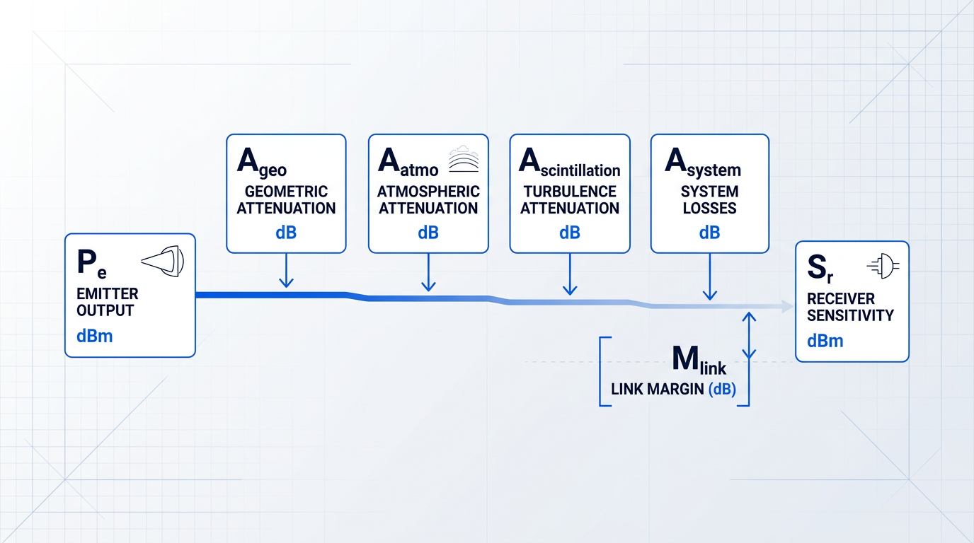
The same general equation form applies whether the link is a short terrestrial hop or a satellite ground-station uplink — the terms are identical, but their magnitudes differ substantially between scenarios, as the later sections on scenario-specific parameters explore.
The budget's additive structure dictates how this guide is organised: each subsequent section builds depth on one or more terms in the equation, from transmitter output power through to the integrated margin calculation. The logical starting point is the first term — P_e, the power the transmitter puts into the path before any losses are applied.
Output Power, Beam Divergence, and Aperture Gain
Every free space optical link budget starts from the same point: the power leaving the transmit aperture, expressed in dBm, is the number from which every subsequent loss is subtracted to arrive at link margin.
P_e — the total emitter power in dBm — is the engineer's most direct lever on the budget. Because the link equation is logarithmic, each additional decibel of transmit power adds exactly one decibel of margin headroom, on a one-for-one basis, with no diminishing returns.
That relationship makes transmitter output power uniquely valuable when atmospheric conditions are variable: more P_e translates directly into more headroom to absorb fog, turbulence, or the geometry of a low-elevation satellite pass — a principle the integrated budget analysis in a later section makes quantitative.
Beam Divergence, Aperture, and Wavelength
No real laser beam is perfectly collimated: the cross-section of the beam grows with distance at a rate set by the beam divergence angle θ, typically expressed in milliradians (mrad) for FSO systems, as ITU-R P.1814-1 formalises in its geometric attenuation model.
A narrower θ preserves power density at the receiver aperture over long ranges, which is why FSO systems generally employ divergence angles of a milliradian or less — but a smaller beam footprint at the receiver demands correspondingly tighter pointing accuracy, a trade-off developed fully in the section on pointing and misalignment losses.
The transmit aperture diameter D is the primary mechanical control over divergence: for a diffraction-limited system, θ scales approximately as λ/D, where λ is the operating wavelength. A larger aperture produces a narrower beam and concentrates more power in the far field — but it also increases system size, mass, and the precision demanded of the pointing mechanism.
Wavelength enters the same relationship. Shorter wavelengths yield narrower beams for a given aperture diameter, but 1550 nm has become the dominant FSO wavelength for reasons that go beyond divergence geometry: it sits within an atmospheric transmission window with low gaseous absorption, and it coincides with the gain band of erbium-doped fibre amplifiers.
The EDFA ecosystem at 1550 nm is particularly mature: as SPIE notes, the 1550 nm band is among the most widely explored for FSO owing to the breadth of telecom components available in this regime, giving system designers access to high-power amplification built on decades of development.
Beam Quality, Optical Efficiency, and Real-World Power
The diffraction limit assumes a perfect Gaussian beam, but real sources deviate from this ideal. The M² parameter (beam quality factor) quantifies that deviation: M² = 1 describes a perfect Gaussian TEM₀₀ beam; any value above 1 means the beam diverges faster than the diffraction limit by a factor of M².
In link budget terms, a degraded beam quality effectively multiplies the divergence angle, increasing the beam footprint at the receiver and reducing the power density that the receive aperture intercepts — making M² a transmitter specification with direct dB consequences, not merely a laser quality metric.
Between the laser source and the output aperture, internal optical components — lenses, isolators, fibre couplers, and beam-shaping optics — introduce losses collected under η_T, the transmit optical efficiency, expressed in dB. ITU-R P.1814-1 places these within A_system; the JPL Descanso link equation treats transmit optics efficiency as a distinct multiplicative factor on the transmitted power.
η_T is easy to underestimate: the output power figure on a laser datasheet typically refers to the source output, not the power reaching the aperture after internal routing losses are applied. Budgeting η_T explicitly prevents a systematic overstatement of the effective P_e entering the propagation path.
Woodrow Scientific's EDF-UL EDFA illustrates what these parameters look like in a high-performance ground-station transmitter. The platform delivers 10 W average output power (40 dBm) at 1550 nm, with M² < 1.1 — a beam quality figure close to the diffraction limit that keeps effective divergence tightly controlled and minimises the power density penalty at the receiver.
The platform supports 0–100% power control with less than 2% stability, making P_e a genuinely adjustable variable rather than a fixed system parameter — the architectural expression of the margin-lever principle described above.
A critical differentiator of the EDF-UL design is its single-beam beacon-and-data architecture: amplitude modulation carries the tracking beacon at a low modulation depth and the uplink data above it, both propagating in the same amplified beam. Systems that separate the beacon and data into distinct beams must account for differential pointing error between them; co-propagating both in one beam eliminates that error source entirely.
The platform is configured to the ground station across both hardware and software layers — band, output power, emitter count, and cooling on the physical side; software-selectable waveforms, modulation index, and standards (CCSDS or SDA) on the control side. This depth of end-to-end configurability, built on patented technology developed in-house at Woodrow Scientific's Southampton facility, is what distinguishes a purpose-built amplifier from a catalogue product.
With 0–100% output power control and less than 2% stability, the EDF-UL treats P_e as a dynamic variable. Every decibel of additional transmit power adds one decibel of link margin — so real-time power adjustment is, in effect, real-time margin management against changing atmospheric conditions.
The EDF-UL is CE and UKCA certified and manufactured in the UK by Woodrow Scientific Limited, a company whose fibre-amplifier expertise is rooted in Southampton's Optoelectronics Research Centre — the birthplace of the EDFA.
With the transmitter parameters established — P_e, θ, aperture diameter, M², and η_T — the next question is how the beam divergence angle drives geometric power loss as the beam propagates: that is the subject of the free-space path loss and geometric attenuation analysis that follows.
Free-Space Path Loss and Geometric Attenuation
Every FSO link suffers a loss that no engineering choice can eliminate entirely: the inevitable dilution of optical power as the beam expands across the propagation path. Unlike atmospheric absorption or fog attenuation, this loss is not a weather event — it is pure geometry, present even in a perfect vacuum, and it can only be managed through careful selection of beam divergence and receiver aperture.
The key distinction to establish at the outset is that free-space path loss (FSPL) is not absorption. No photons are destroyed. What happens instead is that the wavefront expands over an ever-increasing spherical surface area, so the power density at any fixed-aperture receiver falls with the square of distance — a consequence of the inverse square law.
The FSPL Formula and Its Physical Meaning
The classical expression for free-space path loss in dB is: L_FS = 20·log₁₀(4πd/λ), where d is the link distance and λ is the optical wavelength, both in the same units.
Physically, this formula represents the ratio of the surface area of a sphere of radius d — over which the transmitted power is spread — to the effective capture area of an isotropic receiving aperture scaled to the wavelength.
The distance dependence is the dominant term: L_FS scales as 20·log₁₀(d), meaning that doubling the link distance adds approximately 6 dB of free-space loss, regardless of wavelength or aperture.
The wavelength dependence is a nuance that catches engineers moving from RF to FSO: shorter wavelengths produce higher FSPL for a given distance, all else equal. At 1550 nm, the wavelength is orders of magnitude shorter than any RF carrier, so raw FSPL figures appear very large — but this is offset by the far narrower beam divergence that optical systems achieve.
The FSO-Native Formulation: Geometric Attenuation
FSPL is an RF-heritage expression, parameterised by wavelength and distance. FSO link budgets are more naturally expressed in terms of the parameters an optical engineer actually controls: beam divergence angle and receiver aperture area. The ITU-R P.1814-1 (2025) Recommendation — the current authoritative standard for terrestrial FSO propagation prediction — defines geometric attenuation as:
A_geo (dB) = 10·log₁₀(S_d / S_capture), where S_d is the surface area of the transmit beam at range d and S_capture is the receiver capture surface in m².
ITU-R P.1814-1 approximates the beam cross-section area at range d as S_d = (π/4)·(d·θ)², where θ is the full-angle beam divergence in mrad and d is the emitter-receiver distance in km.
The divergence angle drives geometric loss directly and non-linearly: doubling θ quadruples S_d, which adds 6 dB to A_geo. This is the same 6 dB rule that governs distance scaling, and it underlines why minimising divergence is as valuable as shortening the link.
The receiver aperture area (S_capture) appears in the denominator — a larger aperture intercepts a greater fraction of the diverging beam, partially compensating for geometric spreading. This connects directly to the receiver parameters treated in §9, and back to §4, where transmit aperture was shown to govern the achievable divergence angle.
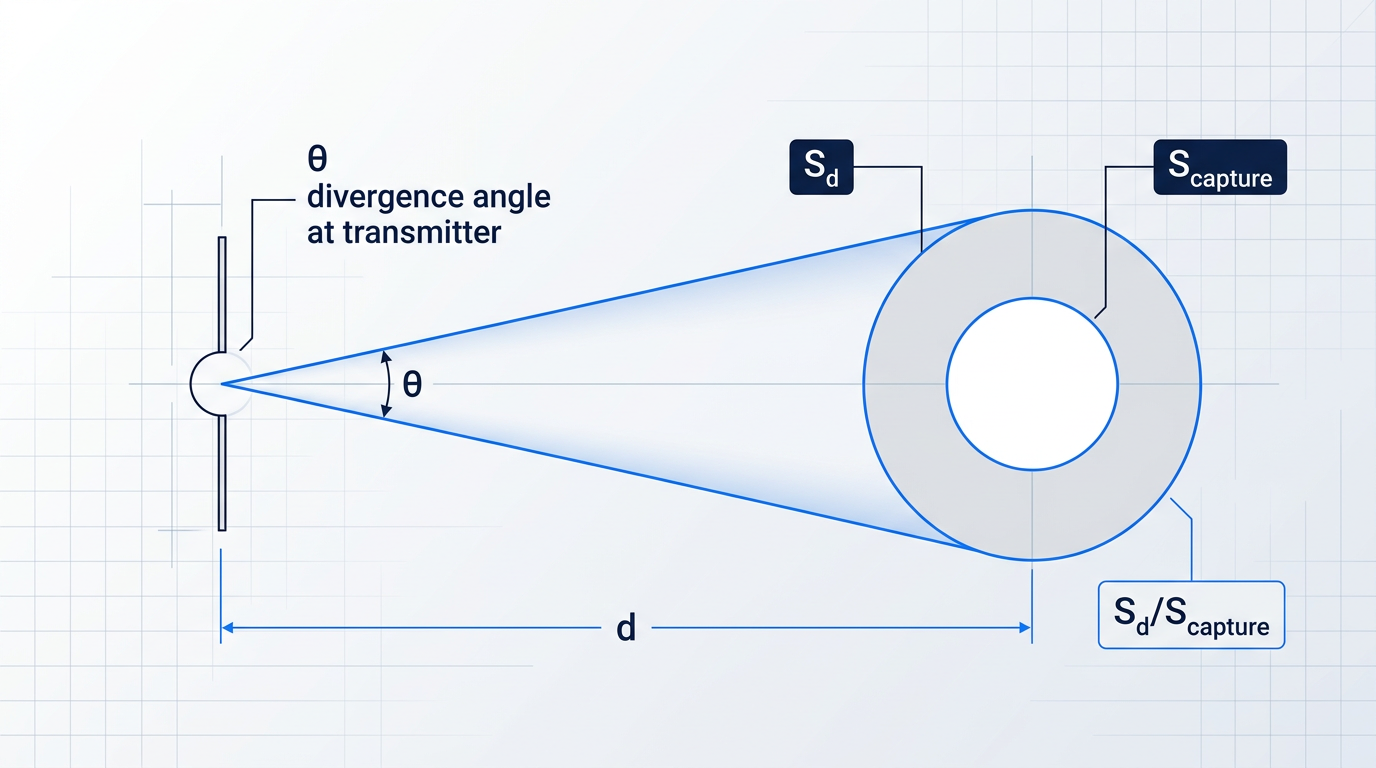
Both FSPL and A_geo describe the same physical mechanism — spreading loss — from different parameterisations. FSPL uses wavelength and distance; A_geo uses divergence and aperture. For FSO design work, A_geo is the more useful form because it maps directly to hardware specifications.
Geometric Loss Magnitude: Worked Examples
ITU-R F.2106-1 provides concrete worked examples that anchor the scale of this loss term. For a link at d = 271 m with a full-angle beam divergence of θ = 4 mrad, the illuminated beam area at the receiver plane is S_trans = 0.92 m², against a receiver capture area of S_capture = 7.85 × 10⁻³ m², yielding A_geo = 10·log₁₀(0.92 / 0.00785) = 20.70 dB.
A separate ITU-R F.2106-1 example using the same 271 m link with θ = 4 mrad and a receiver sensitivity of −50 dBm gives A_geo = 21 dB, producing a link margin of 40.89 dB against a 12 dBm transmit power — illustrating how geometric loss dominates the budget even at sub-kilometre distances when divergence is wide.
These figures make the engineering stakes concrete: at 271 m with a 4 mrad divergence, geometric loss alone exceeds 20 dB. Tightening the divergence angle or increasing the receiver aperture are the two available levers for reducing this term, and both involve hardware trade-offs addressed later in the guide.
Every time the link distance doubles, geometric attenuation A_geo increases by approximately 6 dB. The same 6 dB penalty applies when the full-angle beam divergence doubles. Both relationships follow directly from the 20·log₁₀ scaling in the A_geo formula, making distance and divergence the two most powerful variables in the geometric loss calculation.
FSO vs RF: Beam Narrowness and Its Consequences
FSO systems operate with beam divergence angles typically in the milliradians range — for example, 1.5–6 mrad for commercial terrestrial links. RF antenna beamwidths are measured in degrees, which translates to tens to hundreds of milliradians.
This narrowness concentrates optical power far more effectively over long distances than an RF system of equivalent aperture, producing lower geometric loss for a given link distance. The trade-off is that the narrow beam demands precise pointing and alignment — a sensitivity that grows as divergence is reduced further. That pointing challenge is addressed fully in §8.
In the free space optical link budget, A_geo is the term that contributes this spreading loss to the link margin equation introduced in §3. It is a fixed, deterministic quantity for a given link geometry — unlike the atmospheric terms that follow.
Geometric attenuation sets the irreducible baseline of the loss budget: a function of distance and optics alone, calculable precisely from the system parameters. What follows in §6 is far less predictable — atmospheric attenuation that varies with weather, visibility, and time of day, and which can dwarf geometric loss on terrestrial links.
Atmospheric Attenuation: Absorption, Scattering, Fog, and Rain
With geometric spreading accounted for, the next term to build into the free space optical link budget is the one that most frequently closes — or breaks — a terrestrial link: atmospheric attenuation. Fog, in particular, is the adversary that defines the availability ceiling for ground-level FSO deployments, capable of imposing losses that dwarf every other term in the budget combined.
The Beer-Lambert Law and the Extinction Coefficient
The physical foundation for all atmospheric attenuation calculations in FSO is the Beer-Lambert law, which describes how irradiance decays exponentially with propagation distance through an absorbing and scattering medium.
The governing relationship is I(L) = I(0) · exp(−α · L), where I(0) is the irradiance at the transmitter, I(L) is the irradiance at distance L (km), and α is the total extinction coefficient (km⁻¹) — the single parameter that captures everything the atmosphere does to the beam along the path.
The product α · L is the optical depth of the path: a dimensionless quantity that determines how much of the original irradiance survives. Because the decay is exponential, doubling the path length does not double the loss — it squares the transmission factor, which is why long links under moderate fog accumulate loss far faster than a linear approximation would suggest.
Crucially, α is not a single physical phenomenon. As ITU-R Report F.2106 sets out, the extinction coefficient decomposes into four additive contributions: σ(λ) = αm(λ) + αa(λ) + βm(λ) + βa(λ), where αm is molecular absorption, αa is aerosol absorption, βm is molecular (Rayleigh) scattering, and βa is aerosol (Mie) scattering.
At near-infrared wavelengths — and at 1550 nm in particular — molecular absorption and Rayleigh scattering are small enough to be negligible under most conditions, as ITU-R P.1817 confirms. This means α is dominated by the aerosol terms, and in haze or fog, Mie scattering (βa) becomes the single controlling contribution to the extinction coefficient.
Scattering Regimes and Wavelength Dependence
Which scattering regime applies depends on the ratio of the particle size to the optical wavelength, and that ratio determines whether wavelength selection can help reduce attenuation.
- Rayleigh scattering: Particles much smaller than the wavelength; attenuation scales as λ⁻⁴. Relevant for clear-air molecular scattering but negligible at 1550 nm under most conditions.
- Mie scattering: Particles comparable in size to the wavelength — fog droplets, haze, aerosols. The dominant regime for FSO links; moderately wavelength-dependent.
- Geometric (optical) scattering: Particles much larger than the wavelength — rain drops, snow, heavy fog. Wavelength-independent: the beam is blocked regardless of operating frequency.
ITU-R P.1814 summarises this hierarchy in its Table 1: aerosol and light fog particles (radii 0.005–1 µm) sit in the Mie regime with attenuation scaling roughly as λ⁻¹·⁶ to λ⁰, while heavy fog, rain, and snow particles (radii 1 µm to several mm) fall into the geometric regime where the wavelength dependence is λ⁰ — flat across all FSO operating bands.
The 1550 nm transmission window is chosen because it sits between the water vapour and CO₂ absorption bands, giving low molecular absorption under clear-air conditions — a fact ITU-R P.1814 notes as the basis for selecting near-IR wavelengths for viable FSO links.
Below approximately 500 m visibility, the Kim model's particle-size coefficient q(V) approaches zero, making fog attenuation effectively wavelength-independent. Choosing 1550 nm over shorter wavelengths provides no meaningful advantage once fog is dense enough to push scattering into the geometric regime.
This is a practical engineering constraint, not merely a physics observation: the engineer cannot rely on wavelength selection alone to escape severe fog attenuation, and the link margin must be sized for the fog statistics of the deployment site regardless of the operating wavelength.
Specific Attenuation Across Atmospheric Conditions
To understand why fog dominates the terrestrial FSO link budget, the scale of attenuation across different conditions needs to be seen clearly. ITU-R P.1817 states that attenuation in the optical regime can reach 300 dB/km, and the SPIE Optical Engineering literature records measured peak values above 300 dB/km at 32 m visibility — a figure that makes any link margin calculation based on clear-air assumptions dangerously optimistic.
| Condition | Visibility | Specific Attenuation at 1550 nm (dB/km) | Dominant Mechanism |
|---|---|---|---|
| Clear air | > 50 km | – | Molecular absorption (negligible) |
| Aerosol / light fog | ≳ 0.5 km | – | Mie scattering (aerosol) |
| Heavy / dense fog | ≲ 0.5 km | – | Mie / geometric scattering |
| Extreme fog (measured peak) | ~32 m | > 300 | Geometric scattering |
Specific attenuation at 1550 nm across atmospheric conditions; the measured peak (> 300 dB/km at ~32 m visibility) is from SPIE Optical Engineering. – specific dB/km figures vary with exact visibility and wavelength across the other condition ranges.
The measured extreme of over 300 dB/km at 32 m visibility communicates the essential engineering reality: a path in very dense fog is, for practical purposes, completely opaque, and the ITU-R P.1817 ceiling of 300 dB/km confirms this is not a theoretical edge case.
For satellite FSO links, fog is largely confined to the lowest portion of the slant path and contributes far less to total path attenuation; for terrestrial links, fog is the dimensioning impairment and the link margin calculation must be built around the local fog climate.
Empirical Fog Attenuation Models
Because an analytical approach to Mie scattering requires detailed particle size distributions that are rarely available in practice, the FSO community relies on empirical models that relate specific fog attenuation γ (dB/km) to meteorological visibility V (km). Three models are in common use, each with a distinct applicable range.
Kruse Model
The Kruse model expresses specific attenuation as γ = (3.91/V) · (λ/550)^(−q), where q is a particle-size exponent that varies with visibility range: 1.6 for V > 50 km, 1.3 for 6 km < V < 50 km, and 0.585·V^(1/3) for V < 6 km.
The Kruse model was originally formulated for dust and small aerosol particles significantly smaller than the optical wavelength, with typical diameters around 0.1 µm. As the SPIE literature notes, applying it to fog — whose droplets begin at 2.5 µm diameter and commonly exceed 10 µm — is technically inappropriate, because fog particles are far larger than the wavelength of interest.
In practice, Kruse gives a reliable estimate for visibilities above approximately 650 m, where the aerosol regime holds; below that threshold, it can be overly pessimistic, with actual attenuation values potentially more than 20% lower than the model predicts.
Kim Model
The Kim model addresses Kruse's low-visibility limitation by using a visibility-dependent particle-size coefficient q(V) that correctly captures the weakening wavelength dependence as fog thickens. The functional form uses the same power-law structure, but q(V) transitions through five regimes: 1.6 for V > 50 km, 1.3 for 6 km < V < 50 km, 0.16V + 0.34 for 1 km < V < 6 km, V − 0.5 for 0.5 km < V < 1 km, and q = 0 for V < 0.5 km.
When q = 0, the wavelength term (λ/550)^(−q) collapses to unity and the model becomes wavelength-independent — directly encoding the physical reality that dense fog pushes scattering into the geometric regime. The Kim model is useful as a single-equation fallback when fog type is unknown, particularly across the mid-visibility range, but at very low visibilities the Al Naboulsi model is the more accurate choice, as discussed below.
Al Naboulsi Model
The Al Naboulsi model, developed from FASCOD atmospheric data, provides separate empirical relations for advection fog and radiation fog, covering wavelengths from 690 nm to 1550 nm and visibilities from 50 m to 1000 m.
Advection fog forms when warm, moist air flows over a colder surface, producing droplets with liquid water content above 0.20 g/m³ and mean particle diameters around 20 µm. Radiation fog forms through overnight radiative cooling, with smaller particles (around 4 µm diameter) and liquid water content between 0.01 and 0.1 g/m³. Because these two fog types have different droplet size distributions, they produce different attenuation characteristics at the same meteorological visibility.
For advection fog, the extinction coefficient is σ_advection(λ) = (0.11478λ + 3.8367) / V; for radiation fog, σ_radiation(λ) = (0.18126λ² + 0.13709λ + 3.7502) / V, where λ is in nanometres and V is in metres.
URSI experimental comparisons show the Al Naboulsi model in excellent agreement with measurements at low visibilities, where both the Kruse and Kim models deviate notably from observed data. Use Al Naboulsi when fog type is known from meteorological records and visibility is below 1 km — it is the most physically grounded choice for that regime.
As a practical guide: reach for the Kruse model when visibility exceeds 650 m and fog type is unknown; use the Kim model as a single-equation approach across the mid-visibility range when fog type cannot be identified; and use the Al Naboulsi model when meteorological data identifies the fog type, particularly at the low-visibility end of the range where model accuracy matters most for margin calculations.
Rain Attenuation
Rain occupies a fundamentally different physical regime from fog. Rain droplets (radii 0.1–4 mm) are orders of magnitude larger than the 1550 nm wavelength, placing them squarely in the geometric scattering regime. As ITU-R P.1814 states explicitly, specific rain attenuation is independent of wavelength across the 780–850 nm and 1520–1600 nm FSO transmission windows.
This wavelength independence is a common source of confusion in link budget work: unlike fog, where operating at 1550 nm rather than 850 nm provides some attenuation benefit, rain attenuation is identical across all near-IR FSO bands.
The standard power-law model for rain-specific attenuation is γ_rain = k · R^α (dB/km), where R is the rainfall rate in mm/h and k and α are empirically determined coefficients. The URSI literature cites the Carbonneau relation γ_rain = 1.076 · R^0.67 as a commonly used form.
ITU-R P.1817 makes the scale contrast explicit: in the optical regime, fog attenuation can reach 300 dB/km, while rain attenuation in the millimetre-wave region is typically a few dB/km. For FSO links, rain is significant on long paths or in high-rainfall climates, but it is almost never the dimensioning impairment that fog is. Snow and hail scatter geometrically and are similarly wavelength-independent in FSO bands.
One practical consequence of the complementary nature of these impairments: ITU-R P.1817 notes that hybrid RF/FSO systems can exploit the fact that an RF path is attenuated by rain but largely insensitive to fog, while the optical path is the reverse.
Converting Specific Attenuation to A_atmo
Once γ (dB/km) has been determined from the appropriate model, converting it to the path attenuation term A_atmo that enters the link margin equation is straightforward: A_atmo = γ · L, where L is the link distance in km.
ITU-R P.1814 formalises this for suspended particles (fog, haze) as A_sp = γ_sp · L, noting that the simplest and most practical assumption is that fog concentration is relatively constant along the path. For rain, the same standard introduces a path reduction factor F_rain to account for the spatial inhomogeneity of rainfall, so that the effective rain path attenuation is A_rain = γ_rain · L · F_rain.
In practice, A_atmo is not a single fixed number — it is a random variable whose distribution is driven by the local climate. The engineering question is not what A_atmo is today, but what value it exceeds for what fraction of time at the deployment site.
ITU-R P.1814 provides the standard framework for this analysis: the complementary cumulative distribution function (CCDF) of A_atmo, derived from local visibility and rainfall statistics, maps each attenuation level to the probability it is exceeded. The link margin required to achieve a target availability is read directly from this CCDF. The full statistical methodology is developed in the integrated budget and worked examples later in this guide.
Absorption and scattering remove energy from the beam, or redirect it away from the receiver aperture, producing the deterministic (if climatically variable) loss terms covered here. The next atmospheric impairment is categorically different: turbulence does not remove energy from the path but redistributes it spatially and temporally, adding a time-varying, statistical fading component on top of the attenuation already accounted for.
FSO Solutions Built for Atmospheric Challenges
Atmospheric attenuation is the term that most often breaks a terrestrial link. Our free-space optical communications technology is engineered to help close that margin, even under demanding conditions.

Atmospheric Turbulence: Scintillation, Rytov Variance, Power Fading
Fog and rain remove energy from the optical path — absorption converts photons to heat, scattering deflects them out of the beam. Atmospheric turbulence does neither: it redistributes energy spatially and temporally across the beam cross-section, so the receiver experiences rapid intensity fluctuations rather than a steady reduction in power. This fundamental distinction is what makes turbulence a statistical, time-varying loss term in the free space optical link budget rather than a deterministic attenuation that can be modelled with Beer-Lambert.
The physical mechanism begins with inhomogeneities in atmospheric temperature and pressure, which produce random, spatially and temporally varying fluctuations in the refractive index of air. As the optical beam propagates through these fluctuations, it accumulates random phase perturbations across its wavefront. Those phase perturbations then evolve into intensity fluctuations at the receiver — a phenomenon known as scintillation, and the reason stars appear to twinkle.
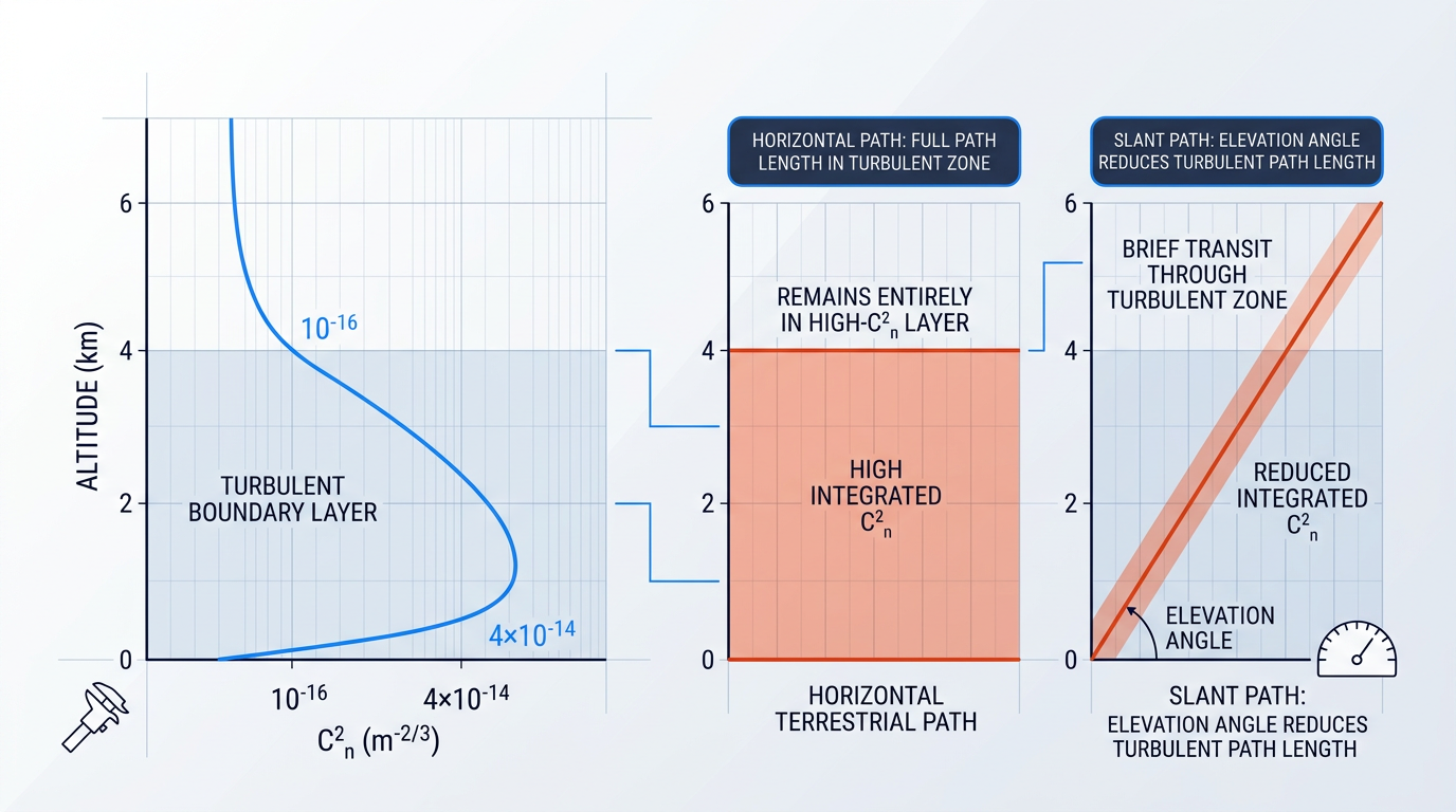
The primary physical quantity that characterises turbulence strength at a given location is the refractive index structure parameter C²_n. Formally, C²_n is the variance of refractive index fluctuations normalised by the separation distance raised to the 2/3 power — the structure constant in the Kolmogorov turbulence model — and carries units of m⁻²/³. Measured values span many orders of magnitude: the UCF dissertations in the FSO literature place typical C²_n values between 10⁻¹⁷ m⁻²/³ for weak fluctuations and 10⁻¹³ m⁻²/³ for strong turbulence conditions.
C²_n is strongly altitude-dependent. NASA measurement campaigns show a clear diurnal cycle near ground level, with C²_n reaching a peak of roughly 4 × 10⁻¹⁴ m⁻²/³ around midday under solar heating and dropping to minimum values near 10⁻¹⁸ m⁻²/³ near sunrise and sunset. Above 4 km, C²_n values generally fall to the range of 10⁻¹⁶ m⁻²/³ or below — a reduction of several orders of magnitude compared to near-ground levels.
For link budget purposes, the integrated turbulence strength along the entire propagation path is captured by the Rytov variance, σ²_R. The formula is σ²_R = 1.23 · C²_n · k^(7/6) · L^(11/6), where k = 2π/λ is the optical wavenumber and L is the path length. Physically, the Rytov variance represents the log-amplitude variance of the optical field under weak perturbation theory.
The exponent on path length — 11/6 — means σ²_R grows rapidly as the link extends: doubling the path length increases the Rytov variance by a factor of roughly 3.6. The weak-turbulence regime is defined by σ²_R < 1; the moderate regime by σ²_R ≈ 1; and strong turbulence by σ²_R > 1. Long horizontal terrestrial paths near the ground can push a link into the strong regime even at moderate C²_n values.
The directly measurable quantity at the receiver is the scintillation index, σ²_I, defined as the normalised variance of received irradiance: σ²_I = (⟨I²⟩ − ⟨I⟩²) / ⟨I⟩². In the weak-turbulence regime, σ²_I ≈ σ²_R, so the two are interchangeable for practical purposes. The distinction matters in strong turbulence: as the Rytov variance exceeds unity, σ²_I saturates and the linear relationship breaks down — the scintillation index reaches a maximum and then gradually decreases toward unity as turbulence grows without bound.
The engineering consequence of scintillation is power fading: rapid, deep drops in received irradiance that can momentarily drive the signal below the detector threshold. NASA technical analyses characterise the typical duration of scintillation-induced temporal fades as on the order of a few milliseconds, with some fades extending as long as 10 ms — long enough to corrupt an entire message packet on a high-data-rate link. The millisecond timescale is fast enough that a link with adequate margin can bridge most fades, but slow enough that forward error correction alone cannot always recover without link-layer retransmission.
The fade statistics are the key input to the link budget. NASA analyses of earth-space optical links show that fade values of 10 dB or larger are observed 12 percent of the time under worst-case turbulence, and 1 percent of the time under weak turbulence. These are the probability-of-exceedance figures that drive the margin calculation.
Turbulence Margin in the Link Budget
In the dB accounting framework of the link budget, turbulence enters as A_scintillation: the fade depth, in dB, that must be covered to achieve a target link availability. The margin is not a fixed attenuation value but a statistical design parameter, read from the tail of the irradiance probability distribution at the desired availability level.
NASA reports on earth-space optical links give concrete reference points: a link margin of 10 dB provides 99% availability, while covering worst-case scintillation to 99.9% availability requires a margin of 20 dB. The gap between those two figures illustrates how steeply the required margin grows as the availability target tightens — an important consideration when specifying A_scintillation for high-reliability links.
NASA earth-space link analyses show that closing the link 99% of the time requires a 10 dB scintillation margin; reaching 99.9% availability under worst-case turbulence demands 20 dB — a doubling of the margin for one extra nine of availability.
Aperture averaging is the most practically accessible technique for reducing the required turbulence margin. When a receiver aperture is larger than the spatial coherence length of the turbulence, it spatially integrates intensity fluctuations across its collecting area, averaging out the rapid spatial variations that a point receiver would see as deep fades. The result is a reduced effective σ²_I compared to a point receiver, quantified by the aperture averaging factor F — the ratio of the normalised intensity variance at a finite aperture to that of a point receiver.
The design implication is direct: a larger receiver aperture reduces A_scintillation, simultaneously increasing collected power and lowering the turbulence margin required to close the link. Theoretical calculations predict an aperture averaging improvement of around 5 dB, with measured field data showing gains as high as 8 dB. This dual role of aperture size — as both a received-power gain term and a turbulence mitigation lever — connects the turbulence margin directly to the receiver aperture design choices covered in the next section.
The contrast between horizontal terrestrial paths and slant paths to satellite is significant for the link budget. The turbulence-generating mechanisms — solar heating, surface convection, and wind shear — are concentrated in the lowest few kilometres of the atmosphere, where C²_n is highest. For a satellite slant path, the beam traverses this turbulent boundary layer only once, at an angle, before entering the comparatively quiescent upper atmosphere.
A horizontal terrestrial link of the same geometric length, by contrast, remains within the high-C²_n near-ground layer for its entire path, accumulating substantially more integrated turbulence. Elevation angle also matters: lower elevation angles increase the slant-path length through the turbulent lower atmosphere, raising the effective integrated C²_n and the resulting Rytov variance. The Hufnagel-Valley model, which expresses C²_n as a function of altitude h, is the standard tool for computing this altitude-weighted path integral for satellite link budgets.
Turbulence is not the only dynamic, probabilistic loss source in the link budget. The beam must also remain precisely aligned with the receiver aperture throughout the link lifetime, and any misalignment — whether from platform vibration, thermal drift, or wind loading — contributes its own statistical loss term. That pointing and misalignment loss is the subject of the next section.
Pointing, Tracking, and Misalignment Losses
Of all the terms in the FSO link budget, pointing loss is the one most likely to be underestimated — and the one that kills links in the field. A beam that arrives at the receiver aperture even slightly off-axis loses power just as surely as if it had passed through heavy fog, and for narrow beams the dB penalty climbs steeply with surprisingly small angular errors.
Pointing loss is the reduction in received power caused by angular misalignment between the transmit beam axis and the centre of the receiver aperture. It is quantified as the ratio of off-axis received power to the peak on-axis power, expressed in dB, and it enters the link margin equation as a component of A_system. It is distinct from geometric path loss — which arises from beam spreading over distance — and from the turbulence-induced scintillation term A_scintillation established in the previous section. With scintillation addressed as a separate budget term, pointing and misalignment losses represent the remaining component of A_system before the full margin equation can be assembled.
Sources of Pointing Error
Pointing error does not arrive from a single source — it is the sum of several physically distinct contributions, each demanding a different engineering response.
- Mechanical jitter: Random, dynamic angular fluctuations driven by building sway, wind loads on the structure, HVAC vibration, and platform motion on mobile systems. The dominant dynamic error source for terrestrial links.
- Boresight bias: A static or slowly varying angular offset between the intended and actual beam axis, caused by thermal or mechanical distortion of the optical mount. Correctable by calibration, but thermal cycling makes it persistent.
- Beam wander: Turbulence-induced displacement of the beam centroid at the receiver plane, introduced in the previous section as a scintillation-related effect. It contributes an equivalent pointing error to the budget.
- ATP residual error: The irreducible angular error remaining after the acquisition, tracking, and pointing system has applied its correction — set by the system's bandwidth, sensor noise, and actuator resolution.
These four sources combine to produce a total angular error at the receiver plane. The Gaussian beam pointing loss model then translates that total angular displacement into a dB loss figure that enters the budget directly.
The Gaussian Beam Pointing Loss Model
For a Gaussian beam, the pointing loss conditioned on radial displacement r from the beam centre is given by h_pl = A_0 · exp(−2r²/w_e²), where A_0 = [erf(υ)]² and w_e is the equivalent beam waist at the receiver.
Each term has a clear physical meaning. A_0 — the fraction of power collected at zero radial displacement — captures the finite aperture effect: even at perfect alignment, a receiver aperture of finite size cannot intercept all the power in a Gaussian beam. The exponential term captures the roll-off as the beam axis moves off-centre: as radial displacement r increases, the fraction of power falling within the aperture falls rapidly, with the rate of roll-off governed by w_e.
The parameter w_e is derived from the beam waist at the receiver and the aperture radius — specifically, υ = √(π·r_a²/2·w_b²), where r_a is the receiver aperture radius and w_b is the beam waist. A larger aperture relative to the beam footprint produces a larger A_0 and a slower roll-off with displacement, which is why a physically larger receive aperture is more tolerant of small pointing errors.
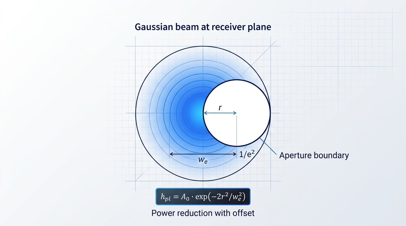
To use the model in a link budget, the engineer converts the total angular pointing error (in μrad) into a radial displacement at the receiver plane by multiplying by the link range, then evaluates h_pl at that displacement and converts to dB. The result is A_system's pointing loss component, ready to subtract from the margin equation.
The DESCANSO Monograph Series 7 (Chapter 5) notes that recent deep-space optical communications link designs have set the total pointing loss allocation at 2 dB, corresponding to a total mispoint angle of 0.42λ/D — where λ is the carrier wavelength and D is the telescope aperture diameter. For a 1064 nm system with a 30 cm aperture, that translates to a total mispoint allocation of 1.5 μrad.
The DESCANSO monograph states that pointing loss and data rate are inversely proportional: a 3 dB decrease in pointing loss equals a 3 dB gain in data rate. Every microradian of improved pointing accuracy is a communications performance gain, not merely a margin reserve.
In practice, the total pointing loss allocation is sub-allocated across error sources: a fraction of the dB budget is assigned to jitter, a fraction to boresight bias, a fraction to thermal and mechanical distortion, and the remainder to the ATP residual. This sub-allocation is not arbitrary — it forces quantitative pointing accuracy requirements onto each subsystem, turning a single dB number into a set of engineering specifications.
The beam divergence trade-off sits at the heart of pointing loss system design. Widening the beam divergence reduces pointing sensitivity — the same angular error produces less power loss because the beam footprint at the receiver is larger — but it simultaneously increases geometric path loss A_geo, because the beam spreads more rapidly over the link distance. Narrowing the divergence preserves power density at the receiver but demands tighter pointing accuracy, raising the pointing loss budget requirement. As the Utah State SmallSat research shows, a 10× reduction in beamwidth can yield a 100× improvement in channel rate — but only if the pointing system can hold the tighter alignment. The engineer must optimise both terms simultaneously; there is no single right answer.
Satellite and Terrestrial Pointing Challenges
The Gaussian beam model applies equally to satellite and terrestrial links, but the dominant error sources and ATP system demands differ substantially between the two scenarios.
For satellite links, the target is moving. Pointing requires ephemeris-driven prediction combined with closed-loop tracking corrections to follow the satellite's angular trajectory as seen from the ground. LEO satellites can require slew rates of approximately 1 degree per second, placing high bandwidth demands on the tracking system. Research on CubeSat optical downlinks shows that fine-stage pointing requirements on the order of ±210 μrad (3σ) are typical for modest-aperture systems, with the beam divergence selected to balance link throughput against the achievable pointing accuracy. After closed-loop correction, the ATP residual error is the dominant remaining pointing error source.
For terrestrial links, the target is fixed — but the transmitter platform is not. Building sway caused by thermal expansion, dynamic wind loads, and weak seismic activity displaces the transmitter beam, introducing misalignment between transmitter and receiver. The ATP system for a terrestrial link is conceptually simpler than its satellite counterpart, but must handle the low-frequency, large-amplitude character of building motion, which differs from the high-bandwidth tracking demands of a moving satellite. The dB loss formulation is identical in both cases; what changes is the statistical character of the angular error feeding into it.
A further pointing error mechanism arises specifically in FSO systems that use a separate tracking beacon beam alongside the data beam. Because the ATP system locks to the beacon, any angular offset between the beacon and the data beam — however small — means the data beam arrives off-axis relative to where the tracking system directed it. This differential pointing error adds directly to the effective misalignment at the receiver and must be carried as an additional term in the pointing loss budget.
The engineering solution is co-propagation: when the tracking beacon and the uplink data share a single amplified beam, the differential pointing error between them is zero by construction. Woodrow Scientific's uplink amplifier platform implements this by nesting the tracking beacon and uplink data in one amplified beam — amplitude modulation carries the beacon at a lower modulation level with the data above it — so the ATP system is locked to exactly the same beam that carries the data, eliminating this error source entirely by design.
Pointing loss completes the loss-side characterisation of the link budget. With geometric spreading, atmospheric attenuation, turbulence-induced fading, and misalignment losses all quantified, the next question is what the receiver does with the power that survives the path — which is the subject of the following section on receiver aperture, sensitivity, and noise.
Receiver Aperture, Sensitivity, and Noise
Every term covered so far — transmit power, geometric spreading, atmospheric absorption, scattering, turbulence, and pointing loss — determines the optical power that arrives at the receiver aperture. What happens at that aperture, and inside the detector behind it, is where the free space optical link budget is ultimately settled: the signal either clears the sensitivity threshold or it does not.
Receiver aperture area (A_R) is the collecting optic's physical area — the cross-sectional area of the telescope, lens, or mirror that intercepts the arriving beam.
As established in §5, geometric attenuation grows because the beam's cross-sectional area expands with distance; A_R is the fraction of that expanded area the receiver actually captures, and it appears on the gain side of the link equation accordingly.
The scaling relationship is direct: received signal power scales linearly with aperture area, which means doubling the aperture diameter quadruples the collected power — a +6 dB gain in the budget.
The DESCANSO Series 7 link equation makes this explicit, with A_R appearing as the numerator of the geometric capture term A_R / (4πz²), confirming that increasing receiver aperture area is one of the most straightforward ways to improve link performance.
Receive optics efficiency (η_R) accounts for the fact that not all power intercepted by the aperture reaches the detector: internal optical elements between the collecting optic and the detector each introduce loss.
The principal contributors include primary and secondary mirror transmission losses, spectral filter insertion loss (a narrowband filter tuned to the laser wavelength rejects background photons but attenuates the signal), relay optics transmission, fibre coupling loss where the receiver feeds a fibre-pigtailed detector, and polarisation losses from reflection and transmission through polarising elements.
JPL's link budget analysis for ground-based optical receivers budgets receiver optical efficiency losses across these components, with the total receiver optical efficiency appearing as a dB loss term in the margin calculation — it reduces the effective received power below what A_R alone would suggest and must be accounted for explicitly.
In the full link margin equation, η_R is folded into the system loss term A_system: it is a loss, not a gain, and treating it as negligible is a common source of optimistic link closure predictions.
Detector sensitivity (S_r), expressed in dBm, is the minimum optical power at the detector input at which the receiver can recover the signal at a specified bit error rate.
In the link margin equation, S_r appears as a subtraction: it is the zero-margin baseline against which received power is measured. If received power exactly equals S_r, the margin is zero and the link is at the edge of closure; the margin is how much the received power exceeds S_r.
Sensitivity is always specified at a given BER — commonly 10⁻⁹ for optical communications — and at a given data rate; it is not a fixed property of the detector in isolation but a function of operating conditions.
Higher data rates demand more photons per bit to achieve the same BER, which means the minimum required received power rises: sensitivity degrades as data rate increases, with the dBm value becoming less negative (closer to zero).
Modulation format also determines sensitivity at a given BER and data rate, because different formats have different photon efficiency. On-off keying (OOK), differential phase-shift keying (DPSK), and coherent formats each achieve a different minimum photon count per bit — SPIE analyses of DPSK versus OOK in satellite FSO links, for instance, quantify DPSK's advantage as approximately 3 dB over OOK under practical conditions, while coherent PSK with homodyne detection approaches the theoretical sensitivity limit.
The noise mechanisms inside the receiver are what ultimately set the achievable sensitivity, and understanding which source dominates is essential for system design.
- Shot noise: The quantum-mechanical floor arising from the discrete nature of photon detection. A shot-noise-limited receiver is operating at its physical optimum for a given optical power.
- Thermal (Johnson) noise: Generated by load resistance and amplifier electronics. Dominates in direct-detection receivers at lower optical powers and higher bandwidths, giving worse sensitivity than the shot-noise limit.
- Dark current: Leakage current in the photodetector with no incident light. Contributes a signal-independent noise floor that limits sensitivity at very low optical power levels.
- Background light: Ambient photons from the sun, sky, or artificial sources entering the receiver FOV, adding shot noise. Particularly significant for terrestrial FSO and daytime satellite ground links.
Which of these dominates determines whether the system is shot-noise limited or thermally limited, and this sets the achievable sensitivity ceiling. A shot-noise-limited receiver is operating near its physical optimum; a thermally limited one may have headroom for improvement through lower-noise electronics, an avalanche photodiode, or an optical pre-amplifier.
Noise figure (F) quantifies the degradation in signal-to-noise ratio introduced by the receiver electronics, and it sets the thermal noise floor against which the received signal must compete.
The thermal noise power in the receiver is given by P_N = F · k · T₀ · B, where k is Boltzmann's constant (1.38 × 10⁻²³ J/K), T₀ is the reference temperature (typically 290–300 K), and B is the receiver bandwidth in Hz.
A higher noise figure means more noise power added per unit bandwidth: in dB terms, P_N(dBW) = F(dB) + k(dBWs/K) + T₀(dBK) + B(dBHz), where k(dBWs/K) = −228.6 dBWs/K.
Noise figure is one of the parameters that determines S_r: it sets the noise floor the signal must overcome, and it feeds directly into the link budget through the sensitivity threshold.
The receiver field of view (FOV) is the angular acceptance cone of the receiver — the solid angle from which the detector accepts incoming light.
A narrower FOV admits less background light, reducing the background-induced shot noise term and improving daytime sensitivity; this is why reducing the ground receiver's FOV can enhance SNR when pointing close to a bright source such as the Sun.
However, tightening the FOV has a direct cost in pointing accuracy: as discussed in §8, the transmit beam must be aimed more precisely to fall within the acceptance cone, increasing the penalty for any residual misalignment.
This is a genuine engineering tension: the FOV that minimises background noise is not the FOV that relaxes pointing requirements, and the two must be balanced in the system design before the budget is finalised.
A larger receiver aperture delivers a second benefit beyond the gain in collected signal power: aperture averaging, the spatial averaging of turbulence-induced intensity fluctuations across the aperture area.
When the aperture diameter exceeds the spatial coherence radius of the turbulence, intensity fluctuations at different points across the aperture become partially uncorrelated and average out, reducing the effective scintillation index at the detector.
As the University of Maryland FSO turbulence research demonstrates, increasing receiver aperture diameter progressively reduces the normalised intensity variance — the aperture averaging factor — with reductions in scintillation that guide the selection of an optimum aperture size.
A larger receiver aperture simultaneously increases collected signal power (scaling as the square of the diameter) and reduces the effective scintillation index through aperture averaging — meaning the required turbulence margin A_scintillation from §7 shrinks as aperture grows. Both benefits enter the link budget together.
This double benefit connects directly to the A_scintillation term introduced in §7: a larger aperture not only captures more of the geometric beam but also reduces the turbulence margin the budget must carry, improving the overall link margin on two axes simultaneously.
With all receiver-side parameters now defined — aperture area, optics efficiency, detector sensitivity, noise sources, noise figure, field of view, and aperture averaging — the next section assembles the complete link margin equation, applies each of these terms alongside the transmitter and loss parameters established earlier, and works through concrete numerical examples.
Integrating the Link Budget: Margin, BER, and Worked Examples
Every preceding section built one piece of the equation: transmit power, geometric spreading, atmospheric attenuation, scintillation, pointing loss, receiver sensitivity. Those pieces now get assembled — and the dB accounting framework that made each term tractable in isolation makes the assembly straightforward.
The integrated link margin equation, as specified in ITU-R P.1814, is: M_link = P_e − S_r − A_geo − A_atmo − A_scintillation − A_system, where every loss term is a positive quantity in dB subtracted from the transmit power P_e (dBm), and S_r is the receiver sensitivity threshold (dBm) at the target BER.
The sign convention is the key: losses reduce the received power below P_e, and the margin is whatever remains above S_r once all losses are accounted for. A positive M_link means the link closes; a negative value means it does not.
The intermediate quantity is received power P_r = P_e − A_geo − A_atmo − A_scintillation − A_system (all in dB), which, when referenced against the noise power floor, gives the SNR at the detector.
SNR maps to bit error rate (BER) through a modulation-specific expression. For NRZ-OOK — the most widely used FSO modulation format — the relationship is BER = ½ · erfc(√(SNR/2)), where erfc is the complementary error function.
The critical design connection is this: receiver sensitivity S_r is defined at a target BER, typically 10⁻⁹ for practical FSO systems. When S_r appears in the margin equation, the BER requirement is already implicitly encoded — a link with positive M_link at the specified S_r is a link that meets its BER target by construction. Other modulation formats (DPSK, PPM) have different BER-SNR curves, but the link budget framework is identical; only the sensitivity figure changes.
How much margin is enough? The fSONA application note on link margin cites a 3 dB baseline floor as the minimum for any FSO link — a 3 dB margin means the received power is double the minimum required, so the link can tolerate a halving of received power before it fails. The Ohio University thesis on FSO link budgets likewise identifies a positive link margin of 3 dB as the standard protection figure used in practice. Additional fade allowances are layered on top of this baseline to cover turbulence events and severe atmospheric conditions; these are scenario-specific and derived from the CCDF of total atmospheric attenuation rather than from a fixed rule.
Link availability is the fraction of time the margin is positive — the fraction of time the link closes. The required margin to achieve a target availability (99.9%, 99.99%, or higher) is read from the CCDF of total atmospheric attenuation, per ITU-R P.1814. The logic is direct: higher availability targets push further into the tail of the attenuation distribution, where rare but severe events live, and those events demand more margin to survive.
ITU-R P.1814 (updated in 2025 as P.1814-1) provides the statistical framework for combining the CCDFs of suspended-particle attenuation and rain attenuation to obtain the total excess path attenuation distribution. The margin required to meet a given availability target is then read directly from that combined CCDF at the corresponding exceedance probability.
Worked Terrestrial Example
The following walkthrough uses a representative 1 km terrestrial FSO link at 1550 nm, with parameters drawn from published sources: beam divergence θ = 1.5 mrad, transmitter aperture 5 cm, receiver aperture diameter 20 cm, and transmit power P_e = 20 dBm.
A_geo (geometric attenuation, from the beam divergence and aperture treatment in the geometric loss section): with θ = 1.5 mrad and a 20 cm receiver aperture over 1 km, the geometric loss is 11.25 dB, as calculated from the beam footprint-to-aperture area ratio.
A_atmo is evaluated under two conditions. In clear air, the Kim model at 1550 nm gives attenuation below 1.5 dB/km (the Bechtel/fSONA field data places clear-air absorption, urban haze, and smog combined at less than 1.5 dB/km); for this example, 0.43 dB is used for a 1 km clear-air path, consistent with published values at 10 km visibility. Under moderate fog (visibility approximately 1 km), the Kim model yields approximately 15 dB/km, giving A_atmo = 15 dB over the 1 km path.
A_scintillation is assigned from the weak turbulence regime (Rytov variance σ²_R < 1, corresponding to typical near-ground turbulence at 300 ft mounting height). The ASEE FSO design reference gives a representative scintillation loss of approximately 2 dB at 1 km for typical turbulence at moderate mounting height, which is used here.
A_system combines pointing loss and optical efficiency losses. Published FSO link analyses (including the ArXiv NFP study and ASEE reference) use 2 dB for pointing loss and 2 dB for optical losses as representative values for a well-aligned terrestrial link, giving A_system = 4 dB total.
Receiver sensitivity S_r is set at −35 dBm at BER = 10⁻⁹, consistent with published InGaAs-based receiver performance for 1550 nm FSO links at practical data rates.
| Budget Term | Parameter / Value | dB Contribution | Margin (Clear Air) | Margin (Moderate Fog) |
|---|---|---|---|---|
| Transmit power P_e | 20 dBm | +20 dBm | – | – |
| Receiver sensitivity S_r | −35 dBm at BER = 10⁻⁹ | −(−35) = +35 dB | – | – |
| Geometric loss A_geo | θ = 1.5 mrad, D_R = 20 cm, d = 1 km | −11.25 dB | – | – |
| Atmospheric loss A_atmo (clear air) | Kim model, V = 10 km, 1550 nm | −0.43 dB | – | – |
| Atmospheric loss A_atmo (moderate fog) | Kim model, V = 1 km, 1550 nm | −15.00 dB | – | – |
| Scintillation A_scintillation | Weak turbulence, σ²_R < 1, 1 km path | −2.00 dB | – | – |
| System loss A_system | Pointing (2 dB) + optical efficiency (2 dB) | −4.00 dB | – | – |
| Link margin M_link | P_e − S_r − A_geo − A_atmo − A_scintillation − A_system | – | +37.32 dB | +22.75 dB |
Terrestrial FSO link budget at 1 km, 1550 nm, P_e = 20 dBm, S_r = −35 dBm. M_link (clear air) = 20 − (−35) − 11.25 − 0.43 − 2.00 − 4.00 = 37.32 dB. M_link (moderate fog) = 20 − (−35) − 11.25 − 15.00 − 2.00 − 4.00 = 22.75 dB. – indicates an intermediate term, not a standalone margin figure.
Two patterns stand out in these numbers. First, geometric loss dominates the fixed budget: at 11.25 dB, A_geo is the single largest constant term, exceeding scintillation and system losses combined. Second, the shift from clear air to moderate fog costs 14.57 dB of margin — a swing large enough to consume the entire margin of a poorly designed link. The clear-air margin of 37.32 dB is well above any practical threshold, confirming that 20 dBm is a comfortable transmit power for this scenario; the fog-condition margin of 22.75 dB remains strongly positive, meaning this link would survive moderate fog with margin to spare.
Solving for Required Transmit Power Under Fog
Rearranging the margin equation to solve for P_e gives: P_e = M_target + S_r + A_geo + A_atmo + A_scintillation + A_system. This is the direct answer to the question of how much transmit power is needed to close the link at a given margin target.
Substituting the fog-condition values with a target margin of 3 dB: P_e = 3 + (−35) + 11.25 + 15.00 + 2.00 + 4.00 = 0.25 dBm (approximately 1.06 mW). At the 20 dBm transmit power used in the example above, the link has 22.75 dB of margin in moderate fog — far more than the 3 dB minimum. Conversely, if the link were power-constrained to 0.25 dBm, it would just close under moderate fog with no margin to spare.
As fog severity increases, A_atmo rises sharply: the Bechtel/fSONA data shows heavy fog at 30 dB/km and very dense fog at 60–100 dB/km. Substituting 30 dB/km into the same equation gives P_e = 3 + (−35) + 11.25 + 30.00 + 2.00 + 4.00 = 15.25 dBm (approximately 33.5 mW) — a 15 dB increase in required transmit power relative to the moderate-fog case. Each additional dB of fog attenuation demands exactly one additional dB of transmit power to maintain the same margin, making the power budget the most direct engineering lever for terrestrial links in fog-prone environments.
Every additional dB of transmit power adds exactly 1 dB of link margin. No other single design lever — larger aperture, FEC coding gain, site diversity — translates so directly into margin. The link budget makes all of these trade-offs numerically comparable, but transmit power remains the most immediate adjustment available to the system designer.
Satellite Uplink: How the Budget Shifts
Applying the same framework to a satellite uplink reveals a fundamentally different balance of terms. The USU SmallSat link analyses show free-space path loss values of 251–258 dB for LEO distances of 400–1000 km at 1550 nm — geometric attenuation that dwarfs any atmospheric contribution. At these scales, A_geo is not one term among several; it is the budget.
Atmospheric effects are confined to the lowest portion of the slant path, and fog is effectively absent above the boundary layer. The USU SmallSat data places total atmospheric slant-path losses (absorption, scattering, turbulence) at 6–27 dB depending on elevation angle — significant, but secondary to the geometric term. For a satellite uplink, the required transmit power to close the link is therefore driven primarily by geometric loss, not atmospheric attenuation: the opposite dynamic to the terrestrial fog scenario examined above.
The design implication is clear: closing a satellite uplink requires maximising transmit power and aperture gain, minimising beam divergence, and achieving sub-milliradian pointing accuracy. The scenario-specific detail — elevation angle effects, slant-path atmospheric modelling, and ground station diversity strategies — is developed fully in the next section.
See How EDFA Technology Closes the Link
The link margin equation is only as strong as the transmit power behind it. Our free-space optical communications EDFA technology is built to help engineers close that margin under real-world atmospheric conditions.

Satellite, Terrestrial, and Inter-Satellite FSO Budgets
The link margin equation is the same regardless of where you deploy — what changes is which terms dominate the budget and by how much. A satellite ground link, a rooftop-to-rooftop terrestrial hop, and an inter-satellite link all follow the same additive dB accounting: transmit power minus receiver sensitivity minus geometric, atmospheric, scintillation, and system losses. The practical engineering challenge in each scenario is different precisely because the dominant loss terms are different.
Satellite Ground Links
Geometric attenuation is the defining fixed loss in any satellite ground link. LEO satellites orbit at roughly 500–2,000 km, MEO at several thousand kilometres, and GEO at approximately 35,000–40,000 km; at those distances A_geo dwarfs every other term in the budget under clear-sky conditions.
The atmosphere is relevant only in the lowest ~30 km of the slant path; above that altitude, propagation is effectively free-space. This is a structural difference from terrestrial links: the atmospheric budget is compressed into a thin layer at the base of the path rather than distributed across the full link distance.
Slant-path turbulence is substantially weaker than horizontal-path turbulence over the same geometric distance, because the refractive-index structure parameter C²_n falls rapidly with altitude — the beam spends most of its path in the near-vacuum above the boundary layer.
The elevation angle is the critical variable for ground station engineers. Slant-path attenuation scales approximately as 1/sin(θ) for elevation angle θ, so a link at 10° elevation traverses roughly six times the atmospheric path length of a zenith pass. For a LEO pass, the satellite moves continuously through a range of elevation angles, meaning the link budget must be designed for the full arc — not just the peak elevation — with the worst-case margin occurring as the satellite approaches the horizon.
Terrestrial Point-to-Point Links
Over typical terrestrial FSO distances of 200 m to roughly 4 km, geometric attenuation is a manageable term — as established in the path loss section of this guide, geometric losses run from approximately −8.76 dB at 500 m to −28 dB at 5 km. The budget challenge on terrestrial links is not geometry; it is weather.
Fog attenuation is the dominant impairment for terrestrial FSO, capable of reaching hundreds of dB/km in dense conditions — figures already established in the atmospheric attenuation section of this guide. The CableFree FSO resource notes that in very thick fogs, attenuation can exceed 100 dB/km, which against a practical fade margin of 20–30 dB constrains reliable deployment to under 500 m in those conditions.
Rain is a secondary concern by comparison. Because raindrop diameters (200–2,000 μm) are much larger than FSO wavelengths, rain scattering is wavelength-independent and typically produces 1–10 dB/km at moderate rainfall rates — severe enough to matter on long links in high-rainfall regions, but far less disruptive than fog for most deployments.
Inter-Satellite Links
Inter-satellite links operate entirely above the atmosphere, so A_atmo and A_scintillation are zero. The budget is determined by geometric path loss and pointing loss alone — making ISLs the cleanest illustration of what those two terms contribute in isolation.
ISL distances span hundreds to thousands of kilometres for LEO constellation cross-links, with GEO relay links reaching up to approximately 45,000 km. The Space Development Agency's optical communications standard defines ISL connectivity between pLEO satellites separated by up to 5,500 km. Over such distances, even sub-microradian misalignment causes meaningful power loss, placing pointing accuracy requirements among the most demanding in the field — a point that connects directly to the pointing loss analysis covered in the earlier section of this guide.
Comparing an ISL budget to a satellite ground link budget reveals exactly what the atmospheric terms add: cloud blockage risk, turbulence-induced fading, and the 1/sin(θ) elevation penalty are all absent in the ISL case, leaving only geometry and pointing as the engineering levers.
| Scenario | Typical Distance Range | Dominant Loss Term | Atmospheric Contribution | Pointing Requirement |
|---|---|---|---|---|
| Satellite Ground (LEO) | ~500–2,000 km slant | Geometric (A_geo) | Concentrated in lowest ~30 km of slant path; scales as 1/sin(θ) | Moderate; worsens at low elevation angles |
| Satellite Ground (GEO) | ~35,000–40,000 km slant | Geometric (A_geo) | Same slant-path structure; fixed elevation angle simplifies budget | Lower dynamics than LEO; still precision-critical |
| Terrestrial Point-to-Point | ~200 m to ~4 km | Fog attenuation (A_atmo) | Distributed across full path; fog can exceed 100 dB/km | Moderate; alignment maintained against vibration and thermal expansion |
| Inter-Satellite Link (ISL) | ~500–45,000 km | Geometric (A_geo) | Zero — entirely above the atmosphere | Extreme; sub-microradian alignment over thousands of km |
FSO deployment scenarios compared across link distance, dominant loss term, atmospheric contribution, and pointing requirement. GEO relay ISL distances up to ~45,000 km are drawn from published Alphasat TDP1 campaign data.
The table makes the design logic clear: as you move from terrestrial to satellite-ground to ISL, the atmospheric terms diminish and geometric and pointing terms become the sole engineering challenge. For terrestrial designers, the budget is fundamentally a weather-availability problem; for satellite ground station engineers, it is a combination of geometric budget closure and atmospheric margin across the elevation arc; for ISL designers, it is a pointing and power problem in a clean free-space channel.
On a terrestrial FSO link, fog attenuation can exceed 100 dB/km — against a typical fade margin of 20–30 dB, this constrains reliable deployment to under 500 m in the worst conditions. No other atmospheric effect comes close to this magnitude at FSO wavelengths, making fog the single design constraint that separates terrestrial FSO from every other scenario.
Two architectural responses address the scenario-specific margin challenges identified above: ground station diversity for satellite links, and configurable transmitter power for uplinks. Both operate as margin levers at the system level rather than the link level.
Ground station diversity exploits the fact that cloud cover is correlated only within a few hundred kilometres — weather systems operate on scales of many hundreds of kilometres, so geographically separated sites experience statistically independent obscuration events. The CCSDS optical communications green book illustrates the arithmetic directly: a network of nine sites each with 67% individual availability can deliver 96% network availability, and a 10-station network optimised for an L1 orbit achieves approximately 95% cloud-free line-of-sight. Multi-emitter arrays at a single site serve a similar function on the uplink, reducing the scintillation index at the flight terminal through transmitter diversity.
The diversity investment is a design trade-off: additional ground stations reduce the margin the single link must carry, but each site adds infrastructure cost and operational complexity. The right balance depends on the mission's availability target and the cloud climatology of candidate sites.
For satellite uplinks, configurable transmitter power provides a complementary real-time margin tool. As a LEO satellite descends toward the horizon during a pass, the slant-path atmospheric length grows and link margin erodes — the 1/sin(θ) scaling means the budget at 10° elevation is materially worse than at zenith. The ability to increase transmit power continuously as elevation angle decreases allows the ground station to recover that margin in real time, without waiting for atmospheric conditions to improve.
This is the operational expression of the power-as-margin-lever principle established in the transmitter parameters section and quantified in the integrated margin analysis. The WSL EDF-UL, introduced in that earlier discussion, is configured to the ground station's requirements across both hardware and software layers — output power, band, emitter array architecture, and modulation scheme are all set to the client's specification, not selected from a fixed catalogue. Its 0–100% power control with less than 2% stability means the uplink margin can be adjusted continuously across the full elevation arc of a LEO pass, protecting link closure at the angles where atmospheric path length is greatest.
With the link budget framework now applied across all three principal FSO deployment scenarios, the final section consolidates the design implications and points toward the practical next steps for engineers closing their own budgets.
Conclusion
Applying the FSO Link Budget: Design Implications and Next Steps
The methodology built across this guide points to one principle worth holding onto: the free space optical link budget is not a calculation you run once and file away — it is the living framework that makes every design trade-off quantitative, every parameter a lever, and every decision traceable to a single output.
Apply it to your specific scenario, validate your margin against local atmospheric conditions, and revisit it as your link requirements evolve — the budget will tell you exactly where the dBs are going.
FSO Link Budget: Frequently Asked Questions
Practical answers on calculation procedure, margin thresholds, fog model selection, and scenario-specific turbulence treatment — each question answered independently so you can open any item without reading the others.
Start with P_e (transmitter output power in dBm), subtract S_r (receiver sensitivity at the target BER), then subtract each loss term in turn: A_geo (geometric spreading from beam divergence and link range), A_atmo (atmospheric attenuation from visibility and path length using Kim, Kruse, or Al Naboulsi), A_scintillation (turbulence-induced fading via Rytov variance from C²_n, wavelength, and path length), and A_system (pointing loss plus optical system losses). The remainder is the link margin M_link. Because every term is expressed in dB, each can be computed independently and the results simply summed — a geometric spreading loss calculated at the desk can be added directly to a fog attenuation value derived from visibility statistics without any unit conversion. ITU-R P.1814 provides the statistical framework for converting atmospheric terms into availability-weighted attenuation values, which is how the budget connects to a target link availability rather than a single worst-case scenario.
The right margin depends on the scenario and the target availability — there is no single universal threshold. Terrestrial links in fog-prone environments often require 20 dB or higher to achieve availability targets of 99.9% or 99.99%, because fog attenuation can reach tens to hundreds of dB/km and even a short dense-fog event consumes margin rapidly. The required margin is a function of the target availability, the atmospheric statistics of the deployment site, and the link scenario — not a fixed rule. ITU-R P.1814 provides statistical methods for deriving the margin required to achieve a given availability target, using local visibility and rainfall-rate distributions as inputs.
The choice depends on visibility conditions and whether the fog type is known from meteorological data. Kim is the preferred default for low-visibility conditions (below approximately 1 km): its particle-size coefficient correctly captures the behaviour of attenuation in very dense fog, where fog droplet sizes far exceed the laser wavelength and the Kruse formula — designed for different conditions — becomes unreliable. Research into fog propagation at FSO wavelengths confirms that below roughly 500 m visibility, attenuation is effectively independent of wavelength across the 785–1550 nm range. Kruse is reliable for moderate-visibility conditions above approximately 650 m and remains the older, more widely cited model; below that threshold, the ScienceDirect FSO attenuation literature notes it can be overly pessimistic. Al Naboulsi offers separate empirical relations for advection fog and radiation fog, making it the best choice when the fog type is identified from meteorological data. Its relations were developed specifically for FSO wavelengths between 690 nm and 1550 nm and visibilities between 50 m and 1000 m. As a practical rule: use Kim as the default for dense fog, Al Naboulsi when meteorological records identify the fog type, and Kruse for moderate-visibility conditions above ~650 m.
Fog is almost always the more severe impairment for terrestrial FSO links — by a large margin. Rain attenuation at FSO wavelengths falls in the geometric scattering regime: raindrops are much larger than the optical wavelength, so scattering is wavelength-independent and the specific attenuation at moderate rainfall rates is typically in the range of a few dB/km. Fog attenuation at comparable visibility can reach tens to hundreds of dB/km — ITU-R Report F.2106 gives an example where 100 m visibility fog produces attenuation around 180 dB/km. The physical reason is straightforward: fog droplets are small enough to scatter near-IR efficiently through Mie scattering, while raindrops scatter geometrically but at far lower particle density. Snow and haze sit between the two extremes. The practical implication for the link budget is that rain attenuation must be included in A_atmo and is real, but the system design margin is almost always set by the fog scenario. A link designed to handle dense fog will handle rain with margin to spare; the reverse is not true.
The key difference is how C²_n is treated along the path. For terrestrial horizontal links, C²_n is approximately constant at a given height above ground and time of day, so the Rytov variance σ²_R = 1.23 · C²_n · k^(7/6) · L^(11/6) can be evaluated directly using a representative constant C²_n value for the path height and atmospheric conditions. For satellite slant-path links, C²_n decreases rapidly with altitude — NASA NTRS research shows the structure constant spanning nearly four orders of magnitude from ground level to around 1 km altitude, and continuing to fall above that. Using a single constant C²_n for a slant path would therefore overestimate turbulence strength significantly. The correct approach is to integrate C²_n(h) over the altitude profile of the slant path. The Hufnagel-Valley model is the standard tool for parameterising this altitude dependence, expressing C²_n as a function of height with tunable parameters for upper-atmospheric wind speed and ground-level turbulence strength. The practical result: integrated turbulence along a satellite slant path is substantially weaker than along a horizontal terrestrial path of the same geometric length, even when the satellite link covers far greater total distance.
Pointing loss in dB is a direct subtraction from the link margin — every dB of pointing loss reduces the available margin by exactly 1 dB, with no interaction effects. The DESCANSO monograph on deep-space optical communications notes that recent satellite optical link designs set the total pointing loss allocation at 2 dB, corresponding to a total mispoint angle of approximately 0.42λ/D (where λ is the wavelength and D is the aperture diameter). For a 1064 nm system with a 30 cm aperture, that works out to a total mispoint allocation of 1.5 μrad. Tighter pointing accuracy recovers margin that can be applied elsewhere in the budget — to cover additional atmospheric fading or to reduce required transmit power. Conversely, a system with loose pointing performance must compensate with higher transmit power or a larger receiver aperture to maintain the same link margin. Pointing loss is typically allocated as a sub-budget within A_system, with sub-allocations distributed across pointing knowledge jitter, residual tracking error, knowledge bias, and mechanical or thermal misalignment — each sized according to the estimated performance of the pointing subsystem's sensors and control loop.
Yes. Variable transmit power allows a ground station to increase output during atmospheric degradation events — fog, turbulence, cloud-edge scintillation — recovering link margin in real time rather than designing the fixed-power system for worst-case conditions at all times. A transmitter with continuous power control can be operated at reduced output under clear-sky conditions, lowering power consumption, then stepped up as conditions deteriorate. This treats transmit power as a dynamic margin reserve rather than a fixed budget input. The approach is particularly valuable for satellite ground links, where the atmospheric path length changes continuously as the satellite moves through its pass: lower elevation angles mean longer slant paths through the atmosphere and higher losses, and variable power lets the ground station compensate in real time. Variable power complements, rather than replaces, other margin strategies such as aperture averaging and site diversity — the strongest designs combine all three.