

Introduction
Getting a fibre optic link right is an exercise in precision, not optimism — and every assumption left unvalidated is a failure waiting to surface.
This guide is written for network designers and optical engineers who need a thorough, applicable reference for optical link budget calculation.
It moves from foundational concepts through the components of the calculation, into a step-by-step methodology with worked numbers, and then into the real-world factors that push field performance away from datasheet values.
By the end, you will have a process you can apply directly, and a practical framework for diagnosing links that fall short.
TL;DR
A reliable fibre optic link is never an assumption — it is the product of a rigorous budget built from worst-case values, an honest accounting of real-world degradation, and margin that holds when conditions diverge from the datasheet. The difference between a link that lasts and one that fails is almost always traceable to how carefully that budget was constructed.
This article covers:

Optical link budget: definition and core vocabulary
Key budget components: power, sensitivity, losses, margin
Step-by-step calculation with a worked example
Real-world accuracy factors: ageing, temperature, bends
Troubleshooting failures and common calculation mistakes
Optical amplifiers in long-span link planning
What is an Optical Link Budget?
A fibre optic link that fails after installation is far more costly than one that was correctly validated before a single cable was pulled. The optical link budget is the engineering discipline that prevents that outcome — a systematic, quantitative accounting of every optical power gain and loss between the transmitter and receiver, used to determine with confidence whether a link will operate reliably across its full intended lifetime.
Formally, the optical link budget is the complete power balance of a fibre optic communication link: it tallies all sources of loss (and, where present, gain) in the optical path to establish whether sufficient signal power reaches the receiver under all operating conditions.
Two related but distinct terms appear throughout link budget work, and conflating them leads to calculation errors. Understanding the difference is essential before any numbers are applied.
- Power Budget: The arithmetic difference between transmitter output power and receiver sensitivity — the total optical loss the link can tolerate before the signal becomes undetectable.
- Loss Budget: The calculated sum of all individual cable plant losses: fibre attenuation, connector losses, splice losses, and any other passive loss elements in the optical path.
The fundamental viability test is straightforward: the link is viable when the loss budget is less than the power budget, with sufficient system margin remaining to accommodate real-world degradation over the link's operational lifetime.
All power levels in a link budget are expressed in dBm (decibels relative to one milliwatt), while losses and gains are expressed in dB (a dimensionless logarithmic ratio). The practical advantage of this framework is that losses combine by simple subtraction rather than multiplication, which makes the arithmetic of a multi-element optical path tractable and auditable.
A critical distinction separates professional link budget practice from naive calculation: budgets are not computed using nominal or typical component values. The correct approach uses minimum guaranteed transmitter output power and accounts for maximum receiver sensitivity degradation at end-of-life, ensuring the link performs reliably throughout its entire operational lifetime, not merely at the moment of commissioning.
A link budget calculated on typical or nominal values is not a professional budget — it is an optimistic estimate. The engineering standard requires worst-case component values at end of life. System margin is not arbitrary padding; it is the calculated allowance that must survive after every worst-case assumption has already been applied.
In practice, the optical link budget functions as the primary pre-installation validation tool for any fibre link design. Adequate margin confirms the design is sound; insufficient margin signals that the design must be revised before equipment is procured or cable is installed. Critically, a budget that exists only on paper — without subsequent verification against measured field loss — remains an assumption, not a validated design.
The inputs that feed the budget calculation are: transmitter output power, receiver sensitivity, fibre attenuation, connector losses, splice losses, and system margin — each of which carries its own engineering specifications and tolerances.
With the conceptual framework and vocabulary established, the next step is to examine each of those components in detail — understanding what drives their values, how they are specified, and how each contributes to the overall budget.
Key Components of the Optical Link Budget
Every number in an optical link budget traces back to one of a small set of physical components — and getting any one of them wrong, even slightly, can mean the difference between a link that runs reliably for 20 years and one that fails six months after commissioning. The following breakdown covers each component in the order it enters the calculation: the power envelope first, then each loss source, then the safety margin that holds the whole budget together.
The Power Envelope: Transmitter, Receiver, and Available Budget
Transmitter output power is the starting point of the entire calculation — the top of the power envelope available to the link.
The correct value to use is the minimum guaranteed end-of-life average optical power launched into the fibre, expressed in dBm, drawn from the transceiver specification. This is not the nominal or headline launch power that appears at the top of a datasheet — it is the floor the transmitter is specified to deliver after ageing across its full operational lifetime. As the ITU-T Optical Fibre Handbook confirms, transmitter output power is given as a range, with the minimum value accounting for connector degradation, ageing effects, and worst-case operating conditions.
Using the minimum rather than the typical or maximum value is the only defensible engineering approach: a budget built on typical launch power will appear comfortable at commissioning but will erode as the transmitter ages, potentially leaving the link with no margin when it needs it most.
Receiver sensitivity is the mirror image: the minimum average optical power required at the receiver input to achieve the specified bit error rate (BER), evaluated at end-of-life under worst-case conditions.
Per ITU-T G.Sup39, receiver sensitivity is defined as the worst-case, end-of-life minimum acceptable mean received power to achieve a BER of 1 × 10⁻¹², accounting for ageing, temperature margins, receiver connector degradation, and measurement tolerances. If received power falls below this threshold, the link fails. Two points demand attention: first, sensitivity degrades over time, so the budget must use the least sensitive value the receiver will exhibit across its lifetime, not its fresh-from-factory performance. Second, sensitivity is always tied to a specific BER target — changing the target (for example, from 10⁻¹² to 10⁻⁹) changes the number, and mixing BER references across components will produce a budget that is internally inconsistent.
The available power budget follows directly from these two values: it is simply the arithmetic difference between transmitter output power (dBm) and receiver sensitivity (dBm), expressed in dB. This derived quantity sets the ceiling for the entire link — the sum of all loss components plus system margin must remain beneath it for the link to function.
As Lightwave Online's link budget guidance states: available light = minimum transmit power minus minimum receive sensitivity. For example, a transmitter at −10 dBm and a receiver with sensitivity of −33 dBm yields 23 dB of available budget. Every subsequent deduction comes out of that 23 dB.
Loss Components: Fibre, Connectors, and Splices
Fibre attenuation is the dominant loss term for any link longer than a few hundred metres, and it deserves the most careful treatment in the budget.
Attenuation is expressed as loss per unit length (dB/km), caused by absorption and scattering in the glass. It is not constant across wavelengths — it is a function of the operating window, and the choice of wavelength has a major effect on how far a link can reach. The ITU-T G.652 standard (the definitive specification for standard single-mode fibre) sets the maximum cabled attenuation coefficients that govern budget calculations for the most widely deployed fibre type.
| Fibre Type | Standard | Wavelength | Max Attenuation (dB/km) |
|---|---|---|---|
| Single-mode (G.652.B) | ITU-T G.652 | 1310 nm | 0.40 |
| Single-mode (G.652.B) | ITU-T G.652 | 1550 nm | 0.35 |
| Single-mode (G.652.D) | ITU-T G.652 | 1310–1625 nm | 0.40 |
| Single-mode (G.652.D) | ITU-T G.652 | 1530–1565 nm (C-band) | 0.30 |
| Multimode 50/125 µm (OM2) | ITU-T G.651.1 | 850 nm | 3.5 |
| Multimode 50/125 µm (OM2) | ITU-T G.651.1 | 1300 nm | 1.0 |
Comparison of maximum cabled attenuation coefficients across fibre types and wavelength windows, drawn from ITU-T G.652 (2024) and ITU-T G.651.1 (2018), for use in worst-case link budget calculations.
The practical implications of these figures are significant. At 1550 nm, standard single-mode fibre loses no more than 0.35 dB/km — making it the preferred window for long-haul links where reach is the primary constraint. At 1310 nm, the maximum rises to 0.40 dB/km, but this window offers near-zero chromatic dispersion for G.652 fibre, making it the default choice for metro and premises single-mode links. Multimode fibre at 850 nm carries a much steeper penalty — up to 3.5 dB/km — but the short distances involved in data centre and enterprise LAN applications (typically under 550 m) mean that total fibre loss remains modest, and the economics of 850 nm VCSELs make this the dominant choice for those environments.
Total fibre loss for a link is calculated by a straightforward multiplication: attenuation coefficient (dB/km) × link length (km). For a 20 km single-mode link at 1550 nm, that is 0.35 × 20 = 7.0 dB of fibre loss before any connector or splice losses are added. The attenuation coefficient used must be the maximum specified value from the ITU-T G.652 standard or the cable datasheet — not the typical measured value at installation. Measured values at commissioning are invariably better than the specified maximum; budgeting against them leaves no room for the degradation that will occur over the link's lifetime.
Connector losses represent the insertion loss at each mated connector pair — the loss that occurs when two connectors are joined in a mating adapter.
The causes are physical: misalignment of fibre cores, surface contamination, fibre geometry variations, and differences between connector types. High-quality connectors in clean, well-aligned mated pairs typically achieve 0.1–0.5 dB per pair. However, the TIA-568 standard specifies a worst-case budget allowance of 0.75 dB per mated connector pair, and this is the figure engineers must use when budgeting — regardless of connector type or expected installation quality.
Connector loss is the most variable of the passive loss components. A contaminated connector can add several dB of loss; a poorly aligned connector degrades further with each mating cycle. More importantly, connector loss is the component most often undercounted.
Engineers must account for every connector pair in the signal path: the connectors at the transmitter and receiver ends (frequently overlooked), connectors at patch panels, and any intermediate distribution points. The FOA's loss budget guidance is explicit on this point — all connectors in the complete link must be included, not just those in the permanently installed cable plant. Undercounting connectors is one of the most common calculation errors in link budget work, and it is covered in detail in the troubleshooting section of this guide.
Splice losses are distinct from connector losses in both cause and magnitude, and the two must never be conflated in a budget.
A splice is a permanent joint between two fibre sections — either fusion-welded or mechanically joined. Fusion splices, the dominant method in outside plant and long-haul links, achieve typical losses below 0.1 dB, often below 0.05 dB for well-matched fibres. The VIAVI/JDSU Fiber Guide uses 0.05 dB as the representative fusion splice figure in link budget calculations. Mechanical splices are significantly lossier — typically 0.2–0.3 dB — and are used only where fusion equipment is unavailable or for temporary repairs.
| Component | Typical Achieved Loss | Worst-Case Budget Value | Source |
|---|---|---|---|
| Mated connector pair (adhesive/polish) | 0.1–0.5 dB | 0.75 dB per pair | TIA-568 / FOA |
| Fusion splice | < 0.05 dB (well-matched fibres) | 0.1 dB per splice | VIAVI/JDSU Fiber Guide / FOA |
| Mechanical splice | 0.2–0.3 dB | 0.3 dB per splice | TIA-568 / FOA |
Comparison of worst-case budget values versus typical achieved values for connector pairs and splice types, drawn from TIA-568, FOA loss budget guidance, and VIAVI/JDSU Fiber Guide.
The gap between typical and worst-case values is instructive. A fusion splice that achieves 0.05 dB in practice should still be budgeted at 0.1 dB — because the budget must hold across the link's entire lifetime, not just at the moment of installation. For links with both fusion and mechanical splices, calculate total splice loss separately for each type (number of fusion splices × worst-case fusion loss, plus number of mechanical splices × worst-case mechanical loss) and sum the results. Never apply fusion splice loss values to mechanical splices, and never assume all splices are fusion unless the link design explicitly specifies it.
System Margin: Engineered Safety, Not Optional Padding
System margin is the component most frequently misunderstood, undervalued, or omitted entirely — and that misunderstanding causes real failures.
System margin is a deliberate, calculated safety allowance built into the budget to absorb real-world degradation that nominal component values do not capture. It must cover: transmitter power decreasing with age, receiver sensitivity degrading over time, connector degradation from repeated mating cycles and contamination, unplanned repair splices added during the link's lifetime, and environmental variation including temperature cycling and physical stress. These are not hypothetical risks — they are certainties for any link operated over a multi-year lifespan.
The professional standard is 3–6 dB of system margin for premises and metro links. ITU-T G.955 confirms that a minimum margin of 3 dB is appropriate for systems using temperature-stabilised lasers and PIN detectors in a typical station environment, with the standard explicitly noting that greater margins are necessary for systems using LEDs, non-temperature-stabilised lasers, or systems operating in outdoor environments. The ITU-R BT.1367 standard similarly recommends a 3–6 dB contingency for fibre optic transmission links.
System margin is deducted from the available power budget before comparing against the sum of link losses — it is not an afterthought applied at the end to check whether the link passes. A link budget with insufficient margin will appear viable on paper at commissioning but will fail as components age. Engineers who cut margin to make a marginal link work on paper are not saving cost; they are deferring a failure.
A link budget without adequate system margin (typically 3–6 dB for premises and metro links) is not a conservative budget — it is an incomplete one. The margin exists to absorb component ageing, connector degradation, unplanned repair splices, and environmental variation that nominal values do not capture. Cutting margin to make a marginal link pass on paper sets up a real-world failure.
With each component defined and its worst-case value established — minimum transmitter power, worst-case receiver sensitivity, maximum attenuation coefficient, 0.75 dB per connector pair, splice losses calculated by type, and system margin reserved — the next step is combining them into the link budget calculation itself, including a fully worked numerical example.
How to Calculate an Optical Link Budget
The formula for an optical link budget takes less than a minute to write down — but running it correctly, with the right values and every loss component accounted for, is what separates a link that performs reliably for two decades from one that fails its first winter. This section assembles the equations, explains the professional standard for parameter selection, and walks through a fully worked example on a realistic 20 km single-mode fibre link at 1310 nm.
The Core Equations
Three equations govern every passive single-span optical link budget calculation, and they must be applied in sequence.
Equation 1 — Available power budget: Available Power Budget (dB) = Tx Output Power (dBm) − Rx Sensitivity (dBm)
This is the total loss the link can tolerate before the received signal falls below the threshold for reliable detection.
Equation 2 — Total link losses: Total Link Losses (dB) = Fibre Attenuation Loss + Connector Loss + Splice Loss + Any Other Losses
Every passive element between transmitter and receiver that attenuates the signal must be counted here — including connectors at both ends, patch panel connections, and all fusion splices along the cable route.
Equation 3 — Remaining margin: Margin (dB) = Available Power Budget − Total Link Losses
The link is viable when the remaining margin equals or exceeds the required system margin allowance — typically 3–6 dB in professional outside plant design, as this reserve covers component degradation, additional repair splices, and unforeseen losses over the link's operational lifetime.
A useful derived quantity is the maximum allowable path loss: Max Path Loss (dB) = Tx Power (dBm) − Rx Sensitivity (dBm) − System Margin (dB). This single number is the ceiling that the sum of all link losses — fibre, connectors, splices, and everything else — must collectively stay beneath, and it can be calculated from three datasheet values before the full design is even sketched.
Max Path Loss = Tx Power − Rx Sensitivity − System Margin. This is a direct, calculable ceiling derived from three inputs — if the sum of your link losses exceeds it, no amount of careful installation will save the design.
The Worst-Case Design Philosophy
Before selecting any parameter values, the professional standard must be understood: the calculation must be run with worst-case values throughout, not nominal or typical datasheet figures.
ITU-T G.Sup39 formalises this discipline explicitly: receiver sensitivities are defined as end-of-life, worst-case values taking into account ageing and temperature margins, and transmitter output powers are taken at their guaranteed minimum, not their typical output.
For fibre attenuation, the maximum specified coefficient from ITU-T G.652 applies — not the manufacturer's typical measured value, which will be lower but is not guaranteed over the cable's installed life.
The FOA states this principle directly: do not use the best possible specs for fibre attenuation or connector loss — give yourself margin. A budget calculated on nominal values is not a budget; it is an optimistic estimate that will fail the link at the worst possible moment.
Worked Example: 20 km Single-Mode Link at 1310 nm
The following example uses a standard single-mode fibre link at 1310 nm — the most common scenario for metro and access outside plant design. All parameter values are drawn from ITU-T standards and practitioner references.
| Parameter | Value | Unit | Source / Note |
|---|---|---|---|
| Transmitter output power (minimum) | −3 | dBm | ITU-T G.957 L-4.1 (STM-4 long-haul, 1310 nm) — worst-case minimum |
| Receiver sensitivity (minimum) | −28 | dBm | ITU-T G.957 L-4.1 — worst-case end-of-life value |
| Fibre span length | 20 | km | Realistic metro/access outside plant link |
| Fibre attenuation coefficient at 1310 nm | 0.4 | dB/km | ITU-T G.652.B/D maximum — worst-case cabled value |
| Connector pairs (mated connections) | 4 | pairs | Tx end, Rx end, plus 2 patch panel connections |
| Loss per connector pair (worst-case) | 0.75 | dB/pair | TIA-568 maximum; FOA worst-case budgeting allowance |
| Fusion splices | 6 | splices | Realistic for 20 km OSP link with cable sections joined |
| Loss per fusion splice (worst-case) | 0.3 | dB/splice | ITU-T G.671 / TIA-568 maximum; FOA budgeting convention |
| Required system margin | 4 | dB | Professional practice for OSP links (3–6 dB range) |
Input parameters for the worked optical link budget calculation, showing each component value, unit, and its authoritative source or justification.
The parameter choices above reflect the worst-case design philosophy: the 0.4 dB/km attenuation coefficient is the ITU-T G.652.B/D specified maximum for cabled single-mode fibre at 1310 nm — not a typical measured value, which would be lower. The connector loss of 0.75 dB/pair is the TIA-568 maximum acceptable value, used here because it covers the full range of field-installed connectors including splice-on types. The Tx/Rx pairing (−3 dBm / −28 dBm) comes directly from ITU-T G.957 Table 3 for the L-4.1 STM-4 long-haul application code at 1310 nm, specified as worst-case end-of-life values.
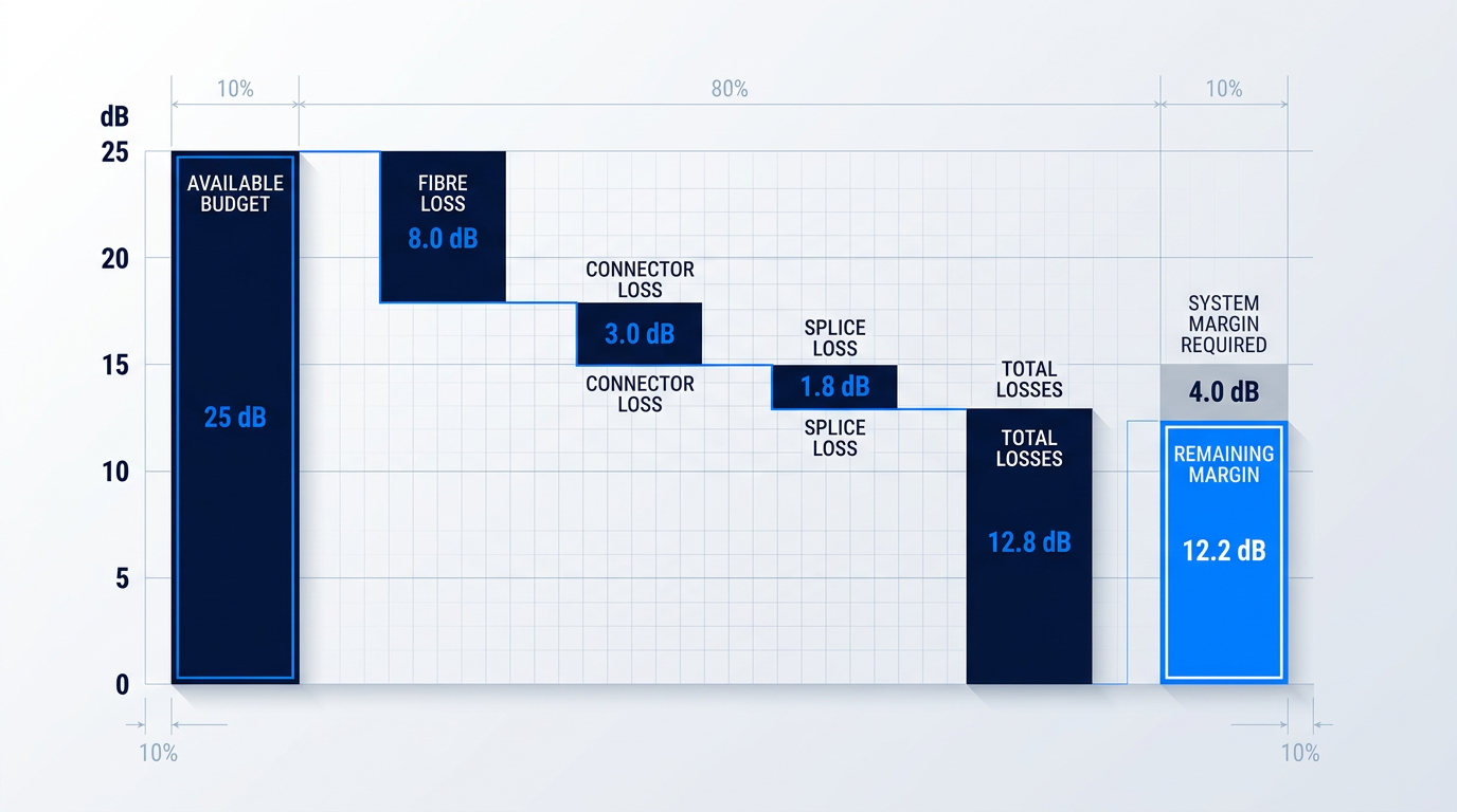
With these inputs, the available power budget is: −3 dBm − (−28 dBm) = 25 dB. This is the design ceiling — the total loss the link must stay beneath to maintain signal integrity.
Step-by-Step Loss Deductions
- Available power budget: Tx power − Rx sensitivity: (−3) − (−28) = 25 dB. This is the total loss the link can absorb.
- Fibre attenuation loss: 0.4 dB/km × 20 km = 8.0 dB. This is typically the largest single loss contributor.
- Total connector loss: 0.75 dB/pair × 4 pairs = 3.0 dB. Includes Tx, Rx, and two patch panel connection points.
- Total splice loss: 0.3 dB/splice × 6 splices = 1.8 dB. Worst-case fusion splice budget per ITU-T G.671 / TIA-568.
- Sum of all link losses: 8.0 + 3.0 + 1.8 = 12.8 dB total link loss.
- Remaining margin: Available budget − total losses: 25.0 − 12.8 = 12.2 dB remaining margin.
- Viability verdict: Remaining margin (12.2 dB) exceeds required system margin (4 dB) by 8.2 dB. Link design is sound.
The verdict is unambiguous: with 12.2 dB of remaining margin against a 4 dB system margin requirement, this link design has substantial headroom — 8.2 dB above the minimum threshold, even after applying worst-case values to every component.
This also confirms the maximum allowable path loss for this transceiver pair: 25 dB − 4 dB (system margin) = 21 dB. The actual link losses of 12.8 dB are well beneath that ceiling, which is why the design passes comfortably.
When the Margin Is Insufficient
Not every link calculation will return a comfortable positive margin. When the remaining margin falls below the required system margin — or turns negative — the design must be revised before deployment.
The available corrective options, in roughly ascending order of cost and complexity, are: shorten the span; reduce the connector count by minimising patch panel hops; specify lower-loss connectors; choose a higher-output transmitter; specify a more sensitive receiver; or, for links where passive design cannot close the budget regardless of component choice, consider optical amplification.
Amplification as an architectural response to budget shortfalls is a distinct engineering discipline — it changes the budget framework fundamentally rather than simply adjusting a loss term — and is addressed separately in the next section.
The Calculation Is a Starting Point
The link budget calculation yields a static design value derived from component specifications on datasheets and standards documents. It is a necessary precondition for deployment — but it is not sufficient on its own.
A budget not verified by field measurement is an assumption. Once the cable plant is installed, OTDR and optical power meter measurements must confirm that actual link losses match the calculated values; any discrepancy signals a problem that requires investigation before the link is commissioned.
The calculation also assumes that component values remain stable — that the fibre attenuation, connector condition, and transceiver performance at installation are the same as they will be in year five or year fifteen. Real links operate in environments where that assumption does not hold, which is why understanding the factors that cause actual performance to diverge from the static calculation is the essential next step.
Real-World Factors That Affect Link Budget Accuracy
The calculation you just completed is correct — and it is not enough. Every value in a static optical link budget is drawn from a datasheet that describes a fibre as it exists on the day it was manufactured, in a controlled environment with no history of mechanical stress or environmental exposure. Real fibre links accumulate all of those things across operational lifetimes measured in decades, and the margin that looked comfortable at commissioning can erode steadily, invisibly, until the link fails.
Four distinct physical mechanisms drive this divergence between the paper budget and field reality. Each one consumes margin that the system margin allowance must absorb — and none of them appear in a nominal datasheet calculation.
Fibre Ageing and Long-Term Attenuation Increase
Fibre attenuation is not a fixed property — it increases over the operational lifetime of the link through several independent mechanisms, any one of which can silently consume margin that the static calculation treats as available.
One of the most consequential is hydrogen ingress: molecular hydrogen diffuses into the fibre core over time, forming OH bonds that introduce absorption peaks at specific wavelengths in the near-infrared. In poorly sealed or damaged cable designs, this process can progress significantly within the link's design life, raising attenuation in the very transmission windows the system depends on.
Outdoor and aerial installations introduce additional ageing mechanisms. UV-induced changes to the fibre coating and glass surface accumulate with prolonged exposure. Sustained mechanical stress — tensile or lateral load on the fibre — promotes microfracture growth that increases scattering loss over time. And coating degradation from combined temperature cycling and UV exposure reduces the protective polymer's ability to isolate the fibre from external lateral forces, progressively increasing the fibre's sensitivity to microbending as the link ages.
The practical consequence is that the attenuation a fibre exhibits at end of life is higher than its commissioning-day figure. Standards-based design practice responds to this by sizing the system margin against worst-case, end-of-life attenuation values rather than the best-case figures a newly manufactured fibre achieves on the test bench. A budget that uses commissioning-day figures as its baseline is, by construction, optimistic.
Temperature Variation and Its Effect on Performance
Both fibre attenuation and chromatic dispersion have measurable temperature dependence, and this matters most in installations where the fibre is exposed to the full range of ambient conditions rather than a thermally controlled indoor environment.
The longer-wavelength transmission windows are disproportionately sensitive to temperature-induced attenuation variation. Aerial spans, direct-buried cables in climates with wide seasonal temperature ranges, and cables traversing thermal gradients all experience effects that are most pronounced in the C-band and L-band — the same windows used by the highest-capacity transmission systems. The 1310 nm window is substantially less affected, which is one reason it remains preferred for shorter, more thermally exposed links.
The fibre coating plays a critical role in this behaviour. As the polymer coating stiffens at low temperatures or softens at high temperatures, its ability to decouple the fibre from external mechanical perturbations changes — with direct consequences for attenuation through increased microbending sensitivity. This thermal cycling effect compounds with the coating degradation mechanism described under fibre ageing: the two are not independent, and their combined effect over time can be larger than either in isolation.
Indoor cables in thermally conditioned environments — data centres, equipment rooms — are largely exempt from these concerns. The practical rule is straightforward: if the cable is outside, or in a space where temperature is not actively controlled, temperature-induced attenuation variation must be explicitly accounted for in the link budget.
Macrobending Loss
When a fibre is bent beyond its minimum bend radius, the evanescent field at the outer edge of the bend can no longer satisfy the conditions for total internal reflection, and optical power leaks from the core into the cladding and radiates away. This is macrobending loss, and its behaviour has two properties that every engineer working with installed cable must understand.
First, the relationship between bend radius and loss is exponential: a modest violation of the minimum bend radius specification causes disproportionately large losses, and small further reductions in radius cause losses that escalate rapidly. A bend that looks physically minor can be optically catastrophic.
Second, macrobend loss is strongly wavelength-dependent. The longer-wavelength windows — C-band at 1550 nm and L-band at 1625 nm — are far more sensitive than the 1310 nm window. A bend radius that causes negligible loss at 1310 nm may introduce significant loss at 1550 nm. This is why bend testing must always be performed at the operating wavelength, not at a shorter wavelength that would yield a falsely optimistic result.
ITU-T G.657 defines a family of bend-loss-insensitive single-mode fibres specifically designed for access network deployments, where tight bends in buildings, cabinets, wall outlets, and distribution points are structurally unavoidable. The standard defines categories with progressively tighter minimum bend radius specifications and correspondingly tighter limits on bend-induced attenuation, addressing a range of deployment scenarios from multi-dwelling units to in-building wiring. The engineering lesson is to specify G.657-category fibre at the design stage in any environment where tight bends are anticipated — not to discover macrobend loss during commissioning or, worse, after deployment.
Macrobending is primarily an installation and specification problem: the mitigation is respecting the cable manufacturer's minimum bend radius and selecting the appropriate fibre category for the environment. Microbending operates through a different mechanism entirely and requires a different engineering response.
Microbending Loss
Microbending refers to small, repeated transverse perturbations along the fibre axis — deviations at a scale far below what the eye can detect, but sufficient to cause mode coupling and optical loss. The sources are structural: lateral pressure from buffer tubes, strength members, and cable jacket; dimensional variations in cable materials as they expand and contract through temperature cycles; and residual stresses in the cable assembly.
Critically, microbending loss is not primarily controlled by installation technique. Unlike macrobending — where careful handling and radius compliance are the main mitigations — microbending is largely determined by fibre and cable design: coating diameter and mechanical stiffness, refractive index profile optimisation, and the structural architecture of the cable itself. The appropriate engineering response is specifying a cable design suited to the installation environment from the outset, such as armoured cable for direct burial or appropriately constructed buffer tube designs for temperature-cycling outdoor deployments.
The spectral signature of microbending loss also differs from macrobending, reflecting the different physical mechanism and the statistical nature of the perturbation distribution along the fibre. This distinction matters when diagnosing underperforming links — a point developed in the troubleshooting section that follows.
Fibre ageing, temperature variation, macrobending, and microbending are not edge cases — they are the normal operating conditions of any outside plant or access network link. A budget calculated from nominal datasheet values cannot see any of them. The margin that appears adequate at commissioning must still be adequate in year fifteen, after each of these mechanisms has been working on it continuously.
A link budget built from typical or best-case component values, with a thin system margin, will pass at commissioning and fail in the field — not because the arithmetic was wrong, but because the arithmetic described a world that does not exist for long.
This is also what makes field failures on apparently well-designed links so difficult to diagnose: the paper budget looked adequate, the commissioning tests passed, and yet the link is underperforming. Knowing how to identify which real-world mechanism is responsible — and how to distinguish a degraded link from a miscalculated one — is the subject of the troubleshooting section that follows.
Optical Amplifiers in Link Budget Planning
There is a point in every long-haul link design where the numbers stop working: span loss exceeds the available power budget, even after system margin has been applied and every real-world degradation factor properly accounted for. At that point, amplification is not a patch — it is an architectural decision that belongs in the design phase, with its own planning framework and its own set of trade-offs.
Introducing an erbium-doped fibre amplifier (EDFA) into a link changes the design calculus in a fundamental way. In a passive link, the dominant noise source is receiver thermal noise and the central question is whether received optical power stays above the receiver sensitivity floor. In an amplified link, the dominant noise source shifts to amplified spontaneous emission (ASE) — generated by the amplifier itself — and the performance metric shifts accordingly, from optical power budget to optical signal-to-noise ratio (OSNR) budget.
In an amplified link, the question is no longer whether the signal arrives above the receiver sensitivity floor — it is whether the signal-to-noise ratio remains adequate after ASE noise accumulates across every amplification stage.
EDFA Placement Configurations
EDFAs are deployed in three distinct configurations, each addressing a different point in the link architecture where gain is needed.
- Booster amplifier: Placed immediately after the transmitter to raise launch power into a long span, extending reach before the signal encounters fibre attenuation.
- In-line amplifier: Placed mid-span to compensate for accumulated fibre loss in multi-span architectures, restoring signal power between transmitter and receiver.
- Pre-amplifier: Placed just ahead of the receiver to lift the incoming signal above the detection threshold, effectively improving receiver sensitivity.
Long-haul systems routinely combine all three: a booster at the transmit end, one or more in-line stages across the span, and a pre-amplifier at the receive end. Each stage is a discrete design decision with its own gain target, noise figure specification, and contribution to the overall OSNR budget.
EDFAs operate across the 1530–1565 nm C-band — the primary gain window, and the region where single-mode fibre attenuation reaches its minimum of approximately 0.2 dB/km — making it the natural home for long-haul amplified links. For capacity-intensive systems, the gain window extends into the 1565–1625 nm L-band, with both bands accessible from a single erbium-doped fibre platform.
Trade-offs in Amplified Link Design
Every amplifier stage adds gain and adds noise. The amplifier's noise figure — typically expressed in dB — characterises how much ASE it contributes relative to the signal. In a multi-span system with several in-line amplifiers, ASE accumulates stage by stage, and the OSNR degrades progressively; the end-of-link OSNR must still meet the receiver's minimum requirement, so each stage's noise figure directly constrains the overall design.
At high launch powers, a second class of constraints becomes relevant: non-linear fibre effects, including self-phase modulation (SPM), cross-phase modulation (XPM), and stimulated Brillouin scattering (SBS). These effects grow with optical power and can degrade signal integrity independently of noise, placing an upper bound on how much gain can be used to compensate span loss. Managing the interplay between OSNR and non-linearity is the central engineering challenge of amplified link design.
For links that require amplification at the leading commercially available power levels — long-haul spans, high-power sensing, or free-space optical applications — a custom-engineered EDFA built to the specific link parameters consistently outperforms a fixed-catalogue module. Woodrow Scientific's Custom EDFA is engineered end-to-end to the application: operating band, output power, pulse regime, cooling, form factor, and control firmware are all configured per project, with average powers above 100 W, peak powers above 100 kW, and pulse energies above 10 mJ at the leading commercially available levels for erbium fibre. As a UK manufacturer that designs, builds, qualifies, and supports its amplifiers in-house on patented technology — with fibre-amplifier expertise rooted in Southampton's ORC, the birthplace of the EDFA — Woodrow Scientific offers a depth of engineering support that catalogue resellers cannot match, covering both C-band and L-band through a single cable.
Whether the link is passive or amplified, the diagnostic approach when a link falls short of its budget follows the same systematic logic — covered in the next section on troubleshooting link failures and common calculation mistakes.
Troubleshooting Link Failures and Common Calculation Mistakes
A link that fails in the field is almost always a calculation error made visible — connectors that were never counted, margin that was trimmed to make the numbers work, bend losses that were present in the installation but absent from the spreadsheet. The diagnostic sequence below is what verification looks like in practice; the common mistakes catalogue is what makes that verification necessary in the first place.
Diagnosing a Link That Falls Short
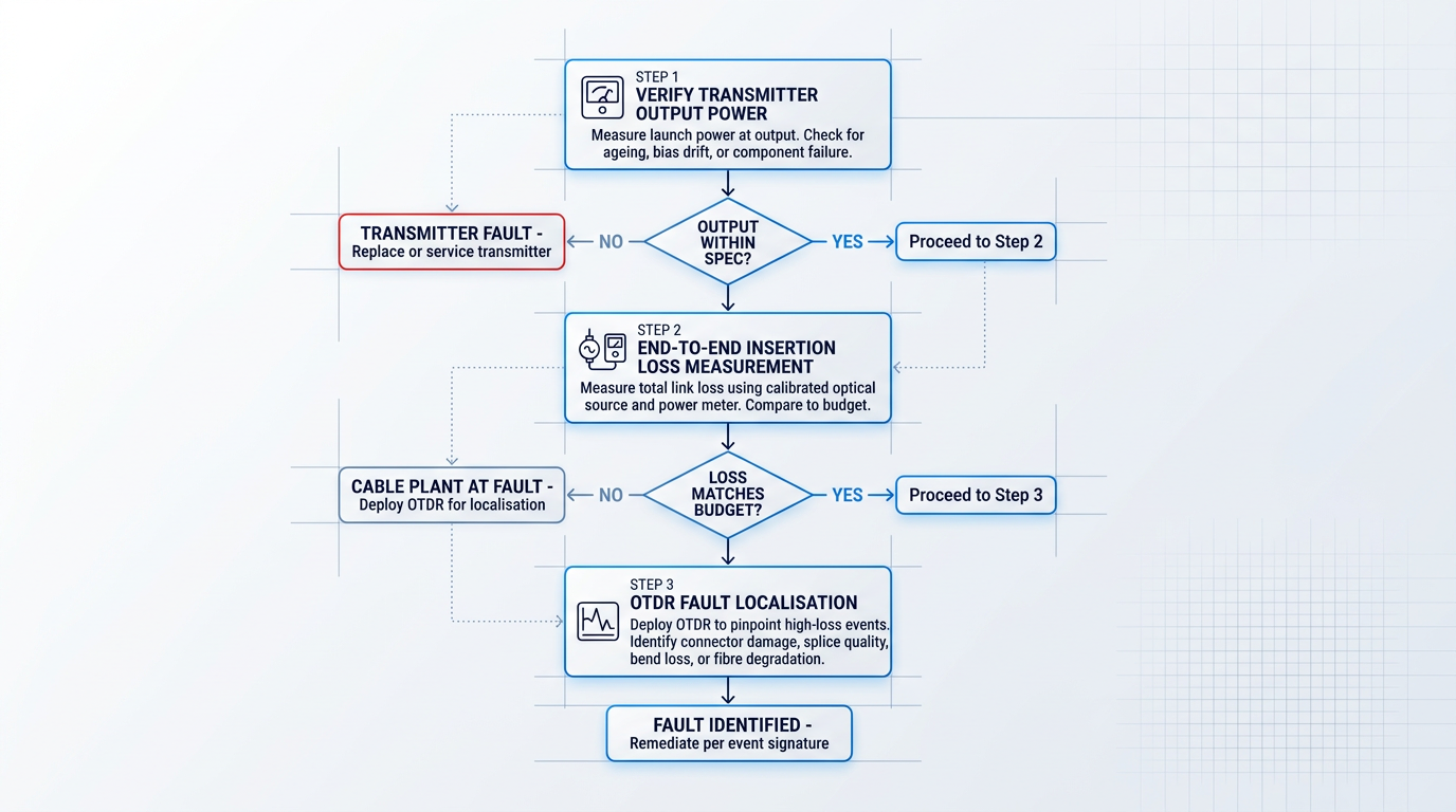
When received power is below prediction, the instinct is often to blame the cable plant immediately — but the fault could be anywhere from the transmitter output to the receiver input. A systematic approach, working outward from the transmitter, isolates the problem efficiently and avoids unnecessary remediation.
- Verify transmitter output power: Measure actual launch power at the transmitter output. Ageing, bias drift, or component failure can reduce output below spec, degrading the entire link before any signal enters the cable plant.
- End-to-end insertion loss measurement: Use a calibrated optical source and power meter to measure total link loss. If measured loss exceeds the budget, the cable plant is at fault. If loss matches but power is still inadequate, revisit transmitter or receiver specifications.
- OTDR to localise high-loss events: Once the cable plant is confirmed as the problem, deploy an OTDR to pinpoint where excess loss is occurring and identify the nature of each event.
Each OTDR trace signature tells a different story: a reflective event with high loss points to a dirty or damaged connector; a non-reflective step loss indicates a poor-quality fusion splice or fibre mismatch; a step loss with no reflection suggests macrobend damage or a crushed fibre; and gradually elevated attenuation across a span signals fibre degradation or sustained environmental stress.
One important discipline: OTDR-measured loss should never substitute for end-to-end insertion loss measurement as the definitive pass/fail verdict. OTDRs can underestimate total link loss — particularly in multimode links — because they measure backscatter, not the actual power a receiver sees. The calibrated source-and-power-meter method is the authoritative check.
Six Common Optical Link Budget Calculation Mistakes
Most link failures that trace back to the calculation share a common root: the budget was built around best-case or nominal values rather than worst-case, end-of-life conditions. The six mistakes below are the specific forms that failure takes — each is recognisable, each is avoidable, and together they account for the majority of optical link budget errors seen in the field.
- Nominal attenuation values: Using a typical figure of 0.2 dB/km at 1550 nm instead of the ITU-T worst-case end-of-life value of 0.275 dB/km produces a budget that passes at commissioning but fails as fibre ages.
- Undercounting connectors: Engineers count connectors in the cable run but miss mated pairs at transmitter and receiver interfaces, inside patch panels, and at wall outlets — every mated pair in the signal path contributes loss.
- Wrong splice loss type: Applying fusion splice loss figures (typically below 0.1 dB) to mechanical splices, which contribute 0.2–0.3 dB each, significantly underestimates total splice loss — an error that accumulates rapidly across many splices.
- Insufficient system margin: Trimming margin below the professional standard of 3–6 dB to make a borderline link viable on paper produces a link that degrades progressively as components age and connectors accumulate wear.
- Ignoring bend losses: Macrobend and microbend losses introduced by installation conditions — common in data centres and access networks — must be explicitly budgeted; unaccounted bend loss can consume several dB of margin invisibly.
- Pristine connector loss values: A connector performing at 0.1–0.2 dB at installation may contribute 0.5 dB or more after years of mating cycles and contamination; end-of-life budgets must reflect degraded, not pristine, performance.
The connector undercounting error deserves particular attention because it is the easiest to make and the hardest to spot in a review. The correct discipline is to trace the full signal path from the transmitter output port to the receiver input port and count every mated connector pair encountered — including those hidden inside equipment racks and patch panels.
The splice type error is similarly insidious: in legacy installations, field-repaired links, or access network deployments, mechanical splices are frequently present alongside or instead of fusion splices, and a budget that assumes fusion loss figures throughout will be optimistic by 0.1–0.2 dB per splice before any other error is introduced.
Each of the six errors above is a specific instance of the same underlying failure: budgeting for how the link performs today rather than how it must perform at end of life. The diagnostic sequence exists to find, in the field, what that optimism cost.
It is worth stating plainly that system margin is not optional padding — it is the quantified allowance for every degradation mechanism the calculation cannot predict precisely: connector wear, fibre ageing, temperature cycling, and the accumulated effect of all the small optimisms that crept into the budget. Cutting it to make a marginal link viable on paper simply defers the failure.
With both the diagnostic sequence and the common mistakes catalogue in hand, the final step is to crystallise these practices into a professional posture that travels with the engineer beyond any single project — which is exactly what the conclusion addresses next.
Conclusion
Applying the Optical Link Budget in Practice
A rigorous optical link budget — built from worst-case component values, with honest accounting for ageing, temperature, and bend losses, and with sufficient system margin — is not the cautious approach; it is the professional standard.
The calculation earns its credibility only when field verification closes the loop: OTDR traces and optical power meter measurements confirm whether the budget reflects physical reality, not just datasheet assumptions.
Commission the link against the budget, record those baseline measurements, and return to the document as the link ages — it is the reference point that makes future troubleshooting tractable and end-of-life planning possible.
Optical Link Budget: Frequently Asked Questions
Practical answers to common questions on optical link budget calculation — covering key terminology distinctions, acceptable received power levels, system margin sizing, WDM link budgeting, OTDR verification limits, and how to account for future repair splices.
The power budget is the arithmetic difference between transmitter output power and receiver sensitivity, expressed in dB — it represents the maximum loss the fibre optic link can tolerate. The loss budget is the calculated sum of all cable plant losses: fibre attenuation, connector losses, splice losses, and any other passive losses. A link is viable when the loss budget is less than the power budget minus the system margin allowance. The two terms are sometimes used interchangeably in informal usage, but treating them as distinct quantities is sound engineering practice. The power budget is fixed by the transceiver pair; the loss budget is the designer's running tally of what the cable plant actually consumes. Keeping them separate makes it immediately clear whether a proposed cable plant design fits within the available headroom.
There is no single universal answer — the acceptable received power range is defined entirely by the transceiver's specification. The received power must exceed the receiver's minimum sensitivity (the floor) and remain below the overload threshold (the ceiling). Typical minimum sensitivity figures vary widely: approximately −14 dBm for short-reach transceivers, down to −30 dBm or lower for long-reach or high-sensitivity designs. These are indicative ranges only — always check the specific transceiver datasheet for the authoritative values. Operating too close to the sensitivity floor, with insufficient margin above it, leaves the link vulnerable to degradation as connectors age and laser output gradually declines. The engineering discipline is to verify received power against the datasheet, not against a generic rule of thumb.
For standard premises and metro fibre optic links, a system margin of 3–6 dB is the widely accepted professional standard. For long-haul links, outside plant installations, or environments with significant thermal variation, a more conservative margin of up to 10 dB is appropriate. The margin must cover everything that degrades the link over its operational lifetime: fibre attenuation increase, laser output degradation, connector contamination from repeated mating cycles, and unplanned repair splices. A margin that appears comfortable at commissioning can be entirely consumed by mid-life if it was sized too thinly. Margin is not optional padding — it is a calculated safety allowance that must be sized against the full end-of-life degradation scenario, not the day-one measurement.
In WDM systems, each wavelength channel must be budgeted individually — the optical link budget is not a single calculation but a per-channel exercise. Two structural differences apply beyond a standard point-to-point link. First, MUX and DEMUX insertion losses must be included in every channel's budget. Passive WDM MUX/DEMUX devices typically introduce 1–12 dB of insertion loss depending on device type and channel count — a figure that engineers accustomed to single-wavelength links frequently underestimate. Second, in amplified WDM systems using EDFAs, the performance framework shifts: the relevant metric becomes the optical signal-to-noise ratio (OSNR) budget rather than the received power budget. Amplified spontaneous emission (ASE) noise accumulates across amplifier stages and becomes the dominant performance constraint. Each of these factors requires explicit treatment in the budget.
OTDR measurements are valuable for localising loss events and estimating individual splice and connector losses, but they should not substitute for end-to-end insertion loss testing using a calibrated optical source and power meter. OTDRs measure loss by analysing backscattered light, which means they can underestimate total link loss — particularly in multimode links, where modal distribution effects complicate the measurement. An OTDR trace shows where losses occur and their approximate magnitude; a calibrated end-to-end power meter measurement shows the actual total loss the signal experiences. Both tools have a role: OTDR for diagnostics and event localisation, calibrated source-and-power-meter for link budget verification. Using an OTDR trace alone as the sign-off measurement is a common mistake that leaves real insertion loss unaccounted for.
The standard practice for outside plant links is to include an explicit allowance for future repair splices within the system margin. A common approach is to budget for 3–5 additional repair splices at the worst-case fusion splice loss value applicable to the link. Outside plant fibre is subject to damage from excavation, weather events, and physical disturbance over its operational lifetime — repair splices are not a hypothetical but a near-certainty on any long link. If this allowance is absent from the budget, each repair splice will consume margin that was assumed available for other degradation factors such as connector ageing or laser output decline. The system margin must be sized to absorb both anticipated component ageing and the repair splice allowance simultaneously — not one or the other.