

Introduction
If you work with fibre optic systems, noise figure appears on every amplifier datasheet, every link budget, and every specification review — often without a clear explanation of what it means for your design.
That gap matters, because noise figure is not a secondary spec you can safely treat as a black box.
It is the parameter that determines how much signal quality your link can preserve, and misreading it leads to decisions that are difficult to unpick once a system is in the ground.
This guide works through EDFA noise figure from the ground up — its physical origins, what drives it, how it behaves across a real system, and what it means for actual design choices.
TL;DR
Noise figure is the single amplifier parameter that sets the OSNR floor for an entire link — and once you understand what physically controls it, you stop reading it as an opaque datasheet number and start using it as a genuine design input.
This article covers:

What EDFA noise figure is and measures
ASE, the 3 dB quantum limit
Gain, pump power, wavelength, operating mode
NF by role: boosters, inline, pre-amps
Cascaded NF accumulation and OSNR
Measurement methods and datasheet conditions
What is EDFA noise figure?
Of all the parameters on an EDFA datasheet, noise figure is the one that sets the ceiling on signal quality. Gain tells you how much the amplifier boosts the signal; output power tells you how hard it can drive the line. But noise figure tells you what the amplifier costs you in signal-to-noise ratio — and that cost is permanent. No amount of subsequent amplification can recover SNR once it has been degraded.
The formal definition
ITU-T G.661, the governing international standard for optical amplifier parameters, defines noise figure (NF) as: the decrease of the signal-to-noise ratio (SNR) at the output of an optical detector with unitary quantum efficiency, due to the propagation of a shot-noise-limited signal through the optical amplifier, expressed in dB.
That definition is precise — but it rewards unpacking. "Unitary quantum efficiency" means an ideal detector that introduces no noise of its own, so any SNR degradation measured at the output is attributable entirely to the amplifier. "Shot-noise-limited signal" means the input signal's noise floor is set by the quantum nature of light itself, not by any classical noise source — in other words, the input is as clean as physics allows.
Stripped to its core: NF is the ratio of input SNR to output SNR, expressed in decibels. A signal enters the amplifier with a certain SNR. It exits with a worse one. The noise figure, in dB, is exactly how much worse.
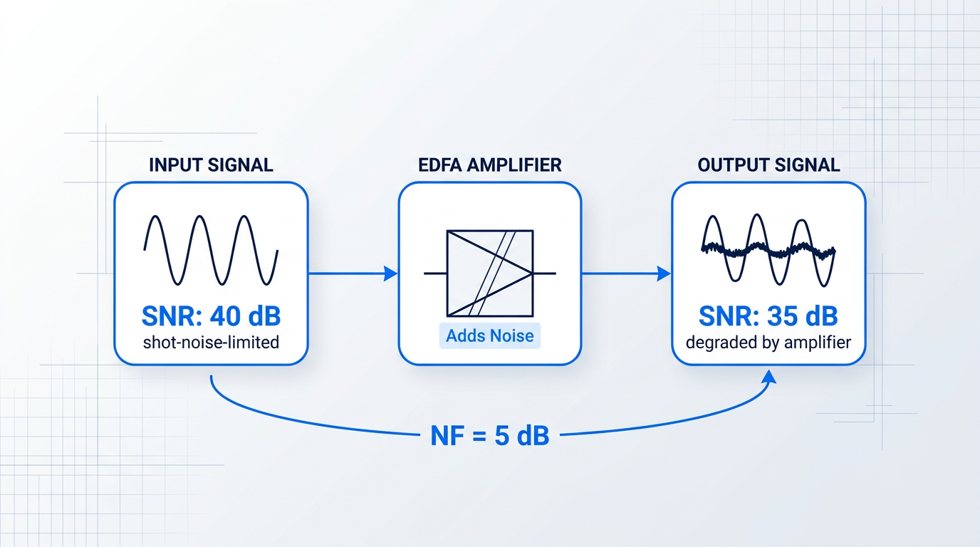
Because an amplifier can only add noise — never remove it — NF is always a positive value (≥ 0 dB by convention, as ITU-T G.661 notes). A lower noise figure means less SNR degradation, which is always better for signal integrity.
Two misconceptions worth clearing up
Noise figure is frequently conflated with two other amplifier parameters. Both confusions lead to misread datasheets and flawed link budgets.
A high-gain amplifier is not automatically a low-noise amplifier. Gain and noise figure are set by different physical conditions inside the amplifier — an amplifier can be engineered for high gain with excellent noise figure, or poor noise figure despite high gain. Always evaluate them as separate specifications.
The second common confusion is between noise figure and output OSNR. NF is the amplifier's contribution to SNR degradation — what the device itself does to the signal. OSNR at the receiver is a system-level result, shaped by NF, input power, gain, and optical filtering bandwidth across the entire link. NF tells you what the amplifier costs; OSNR tells you what the system delivers.
NF requirements by amplifier role
The practical weight of noise figure varies with where in the link an amplifier sits. The weaker the input signal, the more every decibel of NF matters — which is why the three canonical EDFA roles carry very different NF priorities.
- Pre-amplifier (receiver-side): Amplifies the weakest signals, after long spans or high split ratios. NF is the dominant specification — the lowest NF in the system is required here.
- Inline amplifier (line amplifier): Compensates for periodic span loss in long-haul links. NF and output power must both be managed, as noise accumulates across cascaded stages.
- Booster (power amplifier): Placed immediately after the transmitter, where input signals are strongest. Output power is the primary specification; higher NF values are tolerable.
This ordering — pre-amplifier, inline amplifier, booster — runs from most noise-sensitive to least, tracking the strength of the input signal at each position. It is the physical logic that makes noise figure a critical specification in some applications and a secondary one in others.
Typical NF values in commercial EDFAs
The theoretical minimum noise figure for any phase-insensitive optical amplifier is 3 dB — a hard floor set by quantum physics. In practice, commercial EDFAs typically achieve 4–6 dB, with the best designs reaching 4–5 dB, according to UCSB ECE228 lecture data and IEEE TechNav.
Commercial datasheets reflect this range: FS.com inline EDFA products specify NF below 6.0 dB, their booster amplifiers below 6.5 dB, with best-in-class units achieving a typical 4.5 dB. Premlink reports that high-quality EDFAs measured at 0 dBm input achieve 4.0–4.5 dB.
The gap between 3 dB and the 4–6 dB range of real devices is not a manufacturing shortcoming — it is where engineering decisions about pump configuration, fibre design, and operating mode live. Why the 3 dB floor exists, and what drives real amplifiers above it, is the subject of the next two sections.
The definition tells us what noise figure measures. To understand why it has a theoretical minimum and why it varies across devices and operating conditions, we need to look at the physical mechanism generating the noise inside the amplifier itself.
The physical origin of noise figure: amplified spontaneous emission
Before any formula for EDFA noise figure makes sense, you need a physical picture of where the noise actually comes from. The answer is not thermal noise, not electronic interference, and not imperfect engineering — it is a quantum process built into the very mechanism that makes amplification possible: amplified spontaneous emission.
Spontaneous emission in the erbium-doped fibre
When pump light excites Er³⁺ ions into the metastable ⁴I₁₃/₂ energy level, those ions do not simply wait there until a signal photon arrives to trigger stimulated emission.
Any excited ion can decay spontaneously back to the ground state, releasing a photon with random phase, random direction, and a wavelength drawn from the broad fluorescence spectrum of the Er³⁺ transition — spanning a wide band around the signal wavelength, not confined to it.
The pumped fibre is therefore continuously leaking photons in all directions as a natural consequence of its excited state — a behaviour familiar to anyone who has observed a pumped erbium fibre glowing visibly under an infrared viewer.
From spontaneous emission to ASE
Most of those spontaneously emitted photons radiate sideways out of the fibre and are lost — but a small fraction is captured by the waveguide geometry of the fibre core and guided along the fibre in the same modes as the signal.
Once guided, those photons travel through the same gain medium and are amplified by stimulated emission, just like the signal itself.
This is amplified spontaneous emission: the fibre cannot distinguish between a photon that arrived from the transmitter and one that originated from a spontaneous decay inside the gain medium, so both receive the same gain.
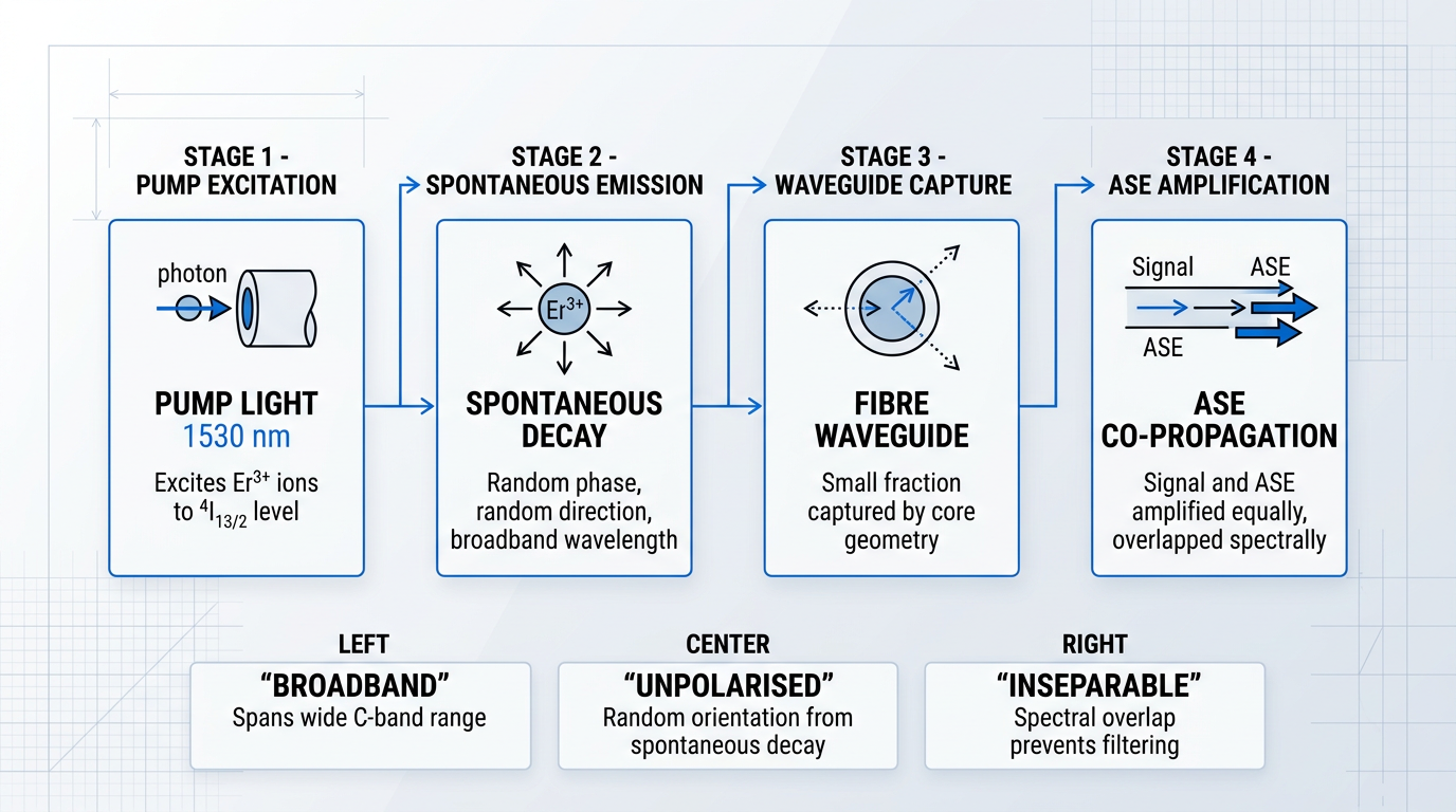
Because spontaneous emission draws from the full fluorescence spectrum of the Er³⁺ transition, ASE is inherently broadband — it spans a wide range across the C-band, not just the signal wavelength.
ASE is also unpolarised, because the direction and polarisation of each spontaneous decay event are random, with no preferred orientation.
The critical practical consequence is that ASE overlaps the signal wavelength spectrally: an optical filter cannot cleanly separate them, because the noise and the signal occupy the same wavelength slot.
When ASE co-propagating with the signal reaches a photodetector, the detector squares their combined optical field, generating a cross-term known as signal-spontaneous beat noise — the dominant noise contribution in a well-designed EDFA.
The spontaneous emission factor and population inversion
The amount of ASE an amplifier generates is not fixed — it depends directly on the degree of population inversion in the gain medium, and this relationship is captured by the spontaneous emission factor, n_sp.
Defined as the ratio N₂/(N₂ − N₁) — where N₂ is the population of the upper laser level and N₁ is the population of the lower laser level — n_sp quantifies how completely the gain medium has been inverted.
When inversion is complete and N₁ approaches zero, n_sp approaches 1, its minimum possible value; when inversion is partial and N₁ is greater than zero, n_sp exceeds 1 and ASE power rises accordingly.
Higher pump power drives higher population inversion, which pushes N1 toward zero, which drives n_sp toward 1, which reduces ASE power, which lowers the noise figure. This chain is not a mathematical abstraction — it is the physical mechanism behind every design decision that affects NF.
Why ASE cannot be eliminated
Spontaneous emission is not an engineering imperfection — it is a fundamental quantum process governed by the physics of the excited state itself, independent of how well the amplifier is designed.
Any medium with population inversion will produce spontaneous emission; any guided spontaneous emission will be amplified; and stimulated emission and spontaneous emission are quantum-mechanically inseparable in any phase-insensitive amplifier.
As RP Photonics states directly: ASE is an unavoidable amplifier noise effect because it arises from the fundamental quantum process of spontaneous emission, and represents a fundamental source of amplifier noise.
There are even fundamental quantum-mechanical reasons why the excess noise of any phase-insensitive optical amplifier — whatever physical principle it is based on — can never be lower than that of an ideal four-level laser amplifier.
Noise components that make up the total NF
The total noise figure of an EDFA is a composite of several distinct noise contributions, each arising from a different interaction between the signal, ASE, and the photodetector.
- Signal-spontaneous beat noise: Beating between the signal and co-propagating ASE at the photodetector. The dominant term in a well-designed amplifier.
- Spontaneous-spontaneous beat noise: ASE beating with itself. Dominant only at very low signal powers; generally negligible in normal operating conditions.
- Shot noise: Intrinsic quantum noise from the signal and ASE photon streams. Usually small relative to the beat noise terms.
Because signal-spontaneous beat noise dominates under normal operating conditions, the EDFA noise figure is fundamentally an ASE story — and n_sp is the key parameter that controls it.
With ASE established as unavoidable and n_sp identified as the quantity that sets its level, the natural next question is: what is the minimum possible value of n_sp, and what noise figure does that imply? That is the question the 3 dB quantum limit answers.
The 3 dB quantum limit and the noise figure formula
ASE explains where the noise comes from — but the deeper question is how much of it there must be, at minimum, in any amplifier, regardless of how well it is designed.
The answer starts with a simple physical argument: at high gain, each signal photon travelling through the erbium-doped fibre stimulates emission, but the excited ions also emit spontaneously into the same amplified mode at a rate that cannot be reduced to zero.
In the best conceivable case — perfect population inversion, every erbium ion in the upper level — the amplifier must still emit at least one spontaneous photon per signal photon into the amplified mode.
That single extra photon per signal photon doubles the noise power in the mode, and a factor of 2 in linear power is exactly 3 dB — the quantum limit for any phase-insensitive linear amplifier, as established by quantum optics.
This is not an engineering approximation or a practical shortfall: it is a fundamental result of quantum mechanics, applying regardless of the physical mechanism providing the gain.
The formal expression makes this precise. In the high-gain limit, the noise figure formula is NF = 2·nsp, where nsp is the spontaneous emission factor introduced in the previous section: nsp = N2/(N2 − N1), with N2 the upper-state population and N1 the lower-state population.
When population inversion is complete — N1 approaches zero, so nsp = N2/N2 = 1 — the formula yields NF = 2·1 = 2, which in decibels is 10·log10(2) ≈ 3 dB.
The high-gain form NF = 2·nsp is the standard engineering expression, but it is an approximation: at finite gain, the full expression includes an additional term that raises NF slightly above 2·nsp, with the correction becoming negligible as gain grows large.
At complete population inversion (nsp = 1), the noise figure formula NF = 2·nsp yields exactly 2 — or 3 dB — the irreducible minimum for any phase-insensitive optical amplifier, set by quantum mechanics, not engineering.
This theoretical expression connects directly to what instruments measure in practice, through the ASE-based optical NF expression used in OSA-based characterisation: NF ≈ PASE / (hν × G × Δν).
In this expression, PASE is the measured ASE power within a bandwidth Δν, hν is the photon energy at the signal frequency, and G is the amplifier gain — all quantities an optical spectrum analyser can measure directly from the output spectrum.
This is the simplified form derived when signal-spontaneous beat noise dominates, and it is the expression used by OSA measurement tools to compute noise figure from a spectral trace — the procedural details of how that measurement is performed are covered later in this guide.
The reason real EDFAs cannot reach 3 dB lies in their quasi-three-level nature: the lower laser level in erbium is also the ground state, so it is never fully depopulated.
Some ground-state erbium ions always absorb signal photons through reabsorption on the signal transition, which means the amplifier must sustain a higher upper-state population to achieve a given net gain than a true two-level system would require.
That elevated upper-state population drives more spontaneous emission, pushing nsp above 1 and therefore lifting NF above 3 dB — not because of poor design, but because of the physics of the erbium transition itself.
In practice, well-designed 980 nm-pumped EDFAs typically achieve noise figures in the range of 4–5 dB; 1480 nm-pumped EDFAs typically achieve 5–7 dB, with 4–5 dB cited as the typical range for optimised EDFAs in the technical literature.
The gap between 3 dB and these practical values is not a failure of real amplifiers — it is the space where engineering decisions live, shaped by quasi-three-level physics, finite gain, and component losses; why 980 nm pumping consistently outperforms 1480 nm on noise figure is explored in a later section.
One further point deserves clarity before moving on: the optical noise figure used in fibre amplifier engineering is not the same quantity as the electrical noise figure used in RF and microwave engineering, even though both share the same name and the same dB unit.
Optical NF is referenced to shot noise — the quantum noise floor of a coherent optical signal — whereas electrical NF is referenced to thermal noise at a standard temperature of 290 K.
Because the two quantities are defined against different noise references, they cannot be directly compared: a 3 dB optical noise figure and a 3 dB electrical noise figure are not the same thing, and treating them as equivalent leads to significant errors in system analysis.
The formula establishes that EDFA noise figure is fundamentally set by nsp — the quality of population inversion throughout the active fibre; the next question is what engineering levers actually control nsp in a real amplifier.
What Controls Noise Figure: Gain, Pump Power, and Inversion
The formula NF = 2·nsp tells you what noise figure is — but it does not tell you what you can do about it. That is the engineer's question: given a target noise figure, which physical knobs actually move it?
The answer reduces to a single governing principle: noise figure is controlled almost entirely by the degree of population inversion at the signal input end of the erbium-doped fibre.
This is worth being precise about. It is not average inversion along the whole fibre that sets NF — it is inversion at the very first point where the signal encounters excited erbium ions.
Because nsp = N2/(N2−N1), a well-inverted input end drives nsp toward 1 and NF toward its 3 dB quantum floor. Every practical lever discussed below — pump power, fibre length, pump direction — acts on noise figure through its effect on that input-end inversion level.
Pump power, fibre length, and the optimum design point
Increasing pump power raises population inversion across the fibre, which pushes nsp lower and brings NF closer to the quantum limit.
The relationship is not linear: improvement is steep at low pump powers and flattens as inversion approaches completeness, because nsp is already near 1 and cannot fall further.
Under-pumping is a practical design failure mode, not just a theoretical concern — an EDFA running with insufficient pump power has measurably elevated ASE, a higher nsp, and a worse noise figure than the same amplifier at its rated pump level.
Fibre length introduces a complementary constraint. Too short a fibre provides insufficient interaction length for the signal to be amplified fully, leaving inversion incomplete and gain low — both of which raise NF.
Too long a fibre creates a different problem: pump power is exhausted partway along the fibre, leaving an unpumped tail where erbium ions sit in the ground state and re-absorb both signal photons and ASE — degrading gain and NF simultaneously.
There is therefore an optimum fibre length for any given pump power and gain target, and it is one of the first parameters a designer fixes when specifying an EDFA.
Why high gain does not guarantee low noise figure
A persistent misconception in EDFA design is that a higher-gain amplifier will automatically have a better noise figure — the reasoning being that both properties improve with stronger population inversion.
The flaw in that reasoning is that gain and noise figure depend on different aspects of inversion: gain reflects total stimulated emission integrated along the full length of the fibre, while NF is set specifically by inversion at the input end.
A high-gain EDFA can have poor noise figure if the signal input end is under-inverted. Conversely, a moderate-gain amplifier with strong input-end inversion can achieve near-quantum-limited NF. Gain tells you about the whole fibre; noise figure tells you about the first few centimetres.
A concrete scenario: if pump power is insufficient to fully invert the fibre from the input end, the signal encounters a weakly inverted medium at the point that matters most for NF — even if enough total gain accumulates downstream to produce an impressive gain figure on the datasheet.
Pump direction: where power lands along the fibre
The direction in which pump light travels through the erbium fibre determines where along that fibre the inversion is strongest — and because input-end inversion governs NF, pump direction has a direct and predictable effect on noise figure performance.
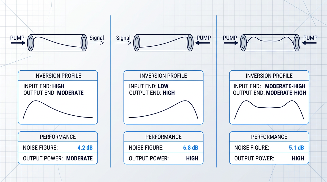
- Co-propagating (forward) pump: Pump and signal travel in the same direction. Pump power is highest at the signal input end, maximising inversion exactly where NF is set. Achieves the lowest noise figure.
- Counter-propagating (backward) pump: Pump enters at the output end. Inversion is highest where the signal is strongest, favouring output power extraction but leaving the input end under-inverted. Results in higher NF.
- Bidirectional pumping: Pumps at both ends simultaneously. Offers a practical compromise: better output power than forward-only, better NF than backward-only, at the cost of a second pump source.
This is a genuine design trade-off with no universally correct answer: co-propagating pumping is the choice when noise figure is the priority, counter-propagating pumping when output power is the priority.
Gain saturation and its effect on noise figure
Noise figure is not a fixed property even for a given amplifier design — it varies with the input signal power.
As input signal power increases and the amplifier approaches gain saturation, stimulated emission from the strong signal partially depletes the population inversion, raising nsp and therefore raising NF.
NF is at its minimum in the small-signal regime — when input power is low enough that the amplifier is operating well below saturation and inversion is largely undisturbed by the signal itself.
This has direct consequences for how different amplifier roles are evaluated: an amplifier running near saturation will exhibit noticeably higher NF than its small-signal specification suggests, a point that becomes important when comparing amplifier types in different network positions.
The pump direction determines where along the fibre pump power is delivered; the pump wavelength determines how completely it can invert the erbium ions — and that distinction carries its own set of noise figure consequences.
Pump wavelength and noise figure: 980 nm vs 1480 nm
The wavelength of the pump laser is not a secondary configuration detail — it sets the noise figure floor of the amplifier before a single metre of erbium fibre has been specified. Get it wrong for your application and no amount of gain optimisation or pump power adjustment will recover the lost performance.
At 980 nm, pump photons carry enough energy to excite Er³⁺ ions to the ⁴I₁₁/₂ energy level — a short-lived excited state well above the signal transition. Fast phonon relaxation drops the ions almost immediately to the metastable ⁴I₁₃/₂ upper laser level, where they accumulate ready for stimulated emission.
Because the 980 nm pump photon energy is well above the signal transition energy, the pump plays no role in stimulated emission on the signal band. Population inversion can therefore approach completeness: nearly all ions sit in the upper state, the spontaneous emission factor nsp approaches 1, and the amplifier approaches the 3 dB quantum limit.
At 1480 nm, the physics is fundamentally different. The pump operates directly on the ⁴I₁₃/₂ metastable level — the same transition the signal uses — so pump photons drive stimulated emission and place a hard ceiling on achievable inversion. Complete population inversion is thermodynamically impossible at 1480 nm; nsp remains greater than 1, ASE power is higher, and the noise figure is correspondingly elevated.
| Parameter | 980 nm Pumping | 1480 nm Pumping |
|---|---|---|
| Noise figure achievable | Lowest achievable — nsp approaches 1, close to the 3 dB quantum limit | Higher — nsp exceeds 1, meaningful NF penalty vs 980 nm |
| Population inversion | Near-complete — pump does not participate in signal transition | Incomplete — pump stimulated emission limits inversion |
| Pump quantum efficiency | Lower — larger quantum defect means more energy lost as heat | Higher — smaller quantum defect, better pump-to-signal conversion |
| Output power capability | Moderate — suited to low-noise stages | High — suited to power-hungry booster stages |
| Primary use case | Pre-amplifiers, low-noise inline amplifiers | Booster amplifiers, high-output-power stages |
Qualitative and structural comparison of 980 nm and 1480 nm pump wavelengths across the parameters that govern EDFA noise figure and power performance.
The noise figure gap between the two pump wavelengths is real and significant for noise-sensitive applications — not a marginal difference that system design can absorb. For pre-amplifier and low-noise inline roles, 980 nm pumping is the only path to noise figures approaching the quantum limit.
The efficiency advantage of 1480 nm pumping is equally real. With a smaller quantum defect, more pump power converts into signal gain rather than heat, giving 1480 nm-pumped stages a genuine edge wherever output power is the primary specification. At high power levels, 1480 nm pump lasers have also historically offered better reliability and lower cost — though that gap has narrowed as high-power 980 nm laser technology has matured.
Many commercial EDFA designs sidestep the trade-off through a dual-stage architecture: a 980 nm-pumped first stage establishes the lowest possible noise figure at the amplifier input, while a 1480 nm-pumped second stage drives output power to the required level. Each stage is optimised for its own function, and the two objectives stop competing.
980 nm and 1480 nm pumping are not points on a continuous dial. They represent fundamentally different interactions with the erbium energy-level structure, and the noise figure consequences follow from that physics — not from pump power settings or fibre length choices made later in the design.
With the pump wavelength decision framed, the next question is what noise figure a given application actually demands — and that depends on the role the amplifier plays in the link. Boosters, inline amplifiers, and pre-amplifiers each carry different NF priorities, which is where the next section picks up.
See Our Custom EDFAs, Built to Your Specification
Pump wavelength sets the noise figure floor before any other design decision is made. Explore our custom EDFAs — engineered from the ground up with the specifications your application actually requires.

Noise Figure by Amplifier Role: Boosters to Pre-Amps
The noise figure requirement for an EDFA is not a fixed target — it depends entirely on where the amplifier sits in the system. The governing principle is straightforward: noise figure matters most when the input signal is weakest, because ASE added to a weak signal degrades the SNR far more severely than the same ASE added to a strong one.
When input signal power is high, the SNR is already well above the noise floor, and a moderately elevated NF has proportionally little impact on the final OSNR. When input power is low, the amplifier's ASE dominates the SNR budget — and any noise added at that point cannot be recovered further downstream.
This single principle generates the entire three-role taxonomy: booster amplifiers see the strongest signals, inline amplifiers see attenuated but not minimal signals, and pre-amplifiers see the weakest signals in the system. The NF requirement tightens as you move from booster to pre-amplifier, in direct proportion to the weakness of the input signal at each position.
| Amplifier Role | Typical Input Power | Primary Specification | Secondary Specification | Typical Noise Figure |
|---|---|---|---|---|
| Pre-amplifier | Very low (after long fibre span or high-loss distribution network) | Noise figure — NF directly sets the SNR floor at the receiver | Gain (high G needed to restore signal before detection) | 4–5 dB; below 4 dB achievable with 980 nm pumping |
| Inline amplifier | Attenuated (span loss compensated periodically) | Balance of NF and output power — both matter in a cascade | Gain flatness across C-band channels | Under 6.0 dB (e.g. FS.com M6200 inline EDFA: under 6.0 dB, 25 dB gain, up to 20 dBm output) |
| Booster amplifier | High (transmitter output, well-defined power level) | Saturated output power (Psat) — drives the first fibre span | Noise figure (secondary; higher NF tolerable here) | Under 6.5 dB (e.g. FS.com M6200-20BA booster: under 6.5 dB, 16 dB gain, up to 20 dBm output) |
Comparison of the three EDFA roles across input power context, primary specification, secondary specification, and typical noise figure — drawing on FS.com commercial datasheets and UCSB ECE228B academic sources.
The table makes the trade-off concrete: moving from booster to pre-amplifier, the primary specification shifts from output power to noise figure, and the NF target tightens by more than 1.5 dB in commercial designs. The half-dB difference between an inline NF of under 6.0 dB and a booster NF of under 6.5 dB may look modest in isolation, but across a cascade of many inline amplifiers that gap accumulates.
Pre-amplifiers: the most noise-critical position
A pre-amplifier receives the weakest signal in the entire link — a signal that has traversed tens of dB of fibre loss, or passed through a high-split-ratio distribution network, before reaching the amplifier input. Because the signal is so weak, the amplifier's ASE is the dominant noise contribution: the NF at this stage sets the effective noise floor of the receiver.
This is why pre-amplifiers demand the lowest NF of any amplifier role, with commercial designs typically specifying NF under 5.5 dB (the FS.com M6200 pre-amplifier specifies under 5.5 dB at 25 dB gain), while the best designs — using 980 nm forward pumping and high population inversion at the input end, as established earlier — can approach or fall below 4 dB.
Output power is a secondary concern for a pre-amplifier: the signal only needs to be raised to a level the receiver can detect, not driven across a long fibre span. This is the application that most strongly motivates 980 nm forward pumping, precisely because complete population inversion at the fibre input minimises nsp and pushes NF toward the quantum limit.
Inline amplifiers: balancing noise and output power
Inline amplifiers (also called line amplifiers) are placed periodically along a long-haul route to compensate for span loss. They receive signals that have been attenuated — typically by 15–25 dB of fibre loss over spans of 40–80 km — but not reduced to the extreme weakness seen at a pre-amplifier input.
Because inline amplifiers cascade across a long link, their noise accumulates: each amplifier adds ASE, and the total OSNR degrades with every additional stage. This means NF cannot be treated as secondary — even a modest NF penalty per amplifier compounds over a chain of ten or twenty spans. At the same time, each inline amplifier must deliver enough output power to drive the next span, so both specifications must be met simultaneously.
A commercial example illustrates the balance: the FS.com M6200 in-line EDFA specifies NF under 6.0 dB with 25 dB gain and up to 20 dBm saturated output power across the C-band. That NF figure is meaningfully tighter than the booster specification, reflecting the cascade sensitivity, while the high output power spec reflects the span-driving requirement.
Booster amplifiers: output power first
A booster amplifier sits immediately after the transmitter, where the signal is at its strongest. Because the SNR at this point is high, a somewhat elevated NF has proportionally little impact on the system OSNR: the noise added by the booster represents a small fraction of the total signal power.
The primary specification for a booster is saturated output power (Psat) — it must launch sufficient power into the first fibre span to ensure the signal survives the attenuation budget to the first inline amplifier or receiver. The FS.com M6200-20BA booster specifies NF under 6.5 dB at 16 dB gain with up to 20 dBm output, illustrating how commercial boosters accept a relaxed NF in exchange for maximising launch power.
The contrast with a pre-amplifier is the clearest expression of the governing principle: the same 20 dBm output power appears in both the booster and the inline datasheet, but the NF target for the booster (under 6.5 dB) is more relaxed than for the inline amplifier (under 6.0 dB) — and both are more relaxed than what a well-designed pre-amplifier achieves.
The two-stage EDFA architecture internalises this role-based principle within a single unit. The first stage is optimised for low NF: high population inversion, 980 nm forward pumping, short erbium-doped fibre, and operation in the small-signal regime. The second stage is optimised for high output power: saturated operation, higher pump power, and often 1480 nm pumping or a longer fibre section. An inter-stage isolator prevents ASE from the second stage from propagating back and degrading the first stage's NF. The architecture does not eliminate the NF-versus-output-power trade-off; it separates the two requirements into distinct stages so each can be independently optimised.
Because noise added to a weak signal cannot be recovered downstream, the pre-amplifier's NF is the single most consequential noise figure in any amplified link. Every 0.5 dB improvement in pre-amplifier NF propagates directly to the system OSNR floor — making it the position where investment in low-NF design pays the highest return.
Understanding which NF is required where is the foundation — but in a real long-haul system, no amplifier operates in isolation. The next question is how NF contributions from many inline amplifiers accumulate across a cascade of spans, and what that arithmetic means for the OSNR budget at the far end of the link.
Noise Figure, Spectral Variation, and Cascaded OSNR
Everything covered so far has treated noise figure as a property of a single amplifier at a single wavelength. That is a useful starting point — but it is not the environment where NF decisions actually have consequences. Real systems have dozens of WDM channels and chains of amplifiers spanning hundreds of kilometres, and in that environment, noise figure behaves in two ways that a single datasheet number cannot capture: it varies across the C-band spectrum, and it accumulates through every amplifier stage in the chain.
The erbium gain spectrum is not flat across the C-band, and because noise figure is tied directly to the gain profile and population inversion distribution along the fibre, NF varies with wavelength in a corresponding way.
The headline NF figure on a datasheet is typically measured at or near 1550 nm — the wavelength where most EDFA designs achieve their lowest NF. Channels at the short-wavelength edge of the C-band, around 1530 nm, experience meaningfully higher NF because reabsorption by ground-state erbium ions is stronger there; channels at the long-wavelength edge face a different but similarly elevated penalty.
In a WDM system, this matters far more than a single-channel view suggests. A channel sitting at the C-band edge does not simply experience slightly worse NF at one amplifier — it accumulates that per-channel NF penalty at every inline amplifier along the link, span after span.
The result is unequal OSNR across the channel comb at the receiver: edge channels arrive with systematically worse signal quality than mid-band channels, even if every amplifier in the chain is nominally identical. The magnitude of that inequality is a direct function of the NF-vs-wavelength curve — a curve that a single headline number cannot represent.
The practical implication for WDM system designers is straightforward: a datasheet NF figure measured at 1550 nm is a best-case, single-wavelength number. When evaluating amplifiers for multi-channel deployments, require the full spectral NF characterisation across the operating band, not just the headline figure.
Noise Figure Accumulation in Cascaded Amplifier Chains
The second dimension of system-level NF behaviour is cascade accumulation. In a long-haul link with N amplifiers, each stage adds ASE noise — and critically, that ASE is then amplified by every subsequent stage in the chain.
The signal does not start fresh at each amplifier. It arrives carrying all the accumulated ASE from every preceding stage, and the next amplifier boosts that noise along with the signal. OSNR at the receiver is therefore a function of the entire chain, not just the final amplifier.
The quantitative framework for this is the Friis formula, expressed in linear (not dB) units: NF_total ≈ NF₁ + (NF₂ − 1)/G₁ + (NF₃ − 1)/(G₁ × G₂) + … Each subsequent amplifier's noise contribution is divided by the cumulative gain of all preceding stages — and that structure encodes an insight far more important than the arithmetic itself.
Consider a first-stage gain of 22 dB, which corresponds to a linear gain of approximately 158×. The second amplifier's NF contribution to the cascade total is divided by 158 — making it, in practice, nearly negligible. A second-stage NF of 5.5 dB adds less than 0.02 dB to the cascade total when the first stage has 22 dB of gain.
With 22 dB of first-stage gain (linear ≈ 158×), the second amplifier's NF contribution to the cascade is divided by 158. Improving NF₁ by 0.5 dB delivers more system benefit than improving NF₂ by 2 dB. The first amplifier in any chain dominates the total noise figure almost entirely — and no subsequent stage can recover what it costs.
This is why pre-amplifiers — which receive the weakest signal after a long span and feed directly into the receiver — are the most noise-sensitive position in any link, as established in the previous section. The Friis formula is the quantitative proof of that intuition: first amplifier dominance is not a design preference but a mathematical consequence of the cascade structure.
As the number of spans grows, OSNR degrades by an additional 10·log₁₀(N) dB relative to a single-amplifier system — so doubling the number of amplifiers costs roughly 3 dB of OSNR, and a tenfold increase costs 10 dB. This makes cascade length one of the most powerful forces acting on receiver signal quality.
Three engineering levers determine OSNR in a cascaded link: amplifier output power (P_out), noise figure (NF), and span loss (fibre attenuation plus connector loss). Of these, output power can be adjusted operationally within limits, and span loss is often fixed by geography and installed infrastructure. Noise figure is the only lever set at amplifier design time — which is precisely why it belongs at the centre of any system specification process.
Understanding that NF varies spectrally and accumulates with every span immediately raises a further question: how is it actually measured, and do two amplifiers with the same datasheet NF number necessarily perform the same way in the field? The answer depends critically on measurement conditions — which is where the next section picks up.
Measuring EDFA Noise Figure: Methods and What They Tell You
You cannot read EDFA noise figure off a single instrument display the way you read output power or gain. NF must be inferred — calculated from the relationship between the ASE power and the amplified signal power measured across the optical spectrum. That inference step is where the complexity lives, and it is why the number on a datasheet is only as trustworthy as the method and conditions used to derive it.
The core measurement challenge is separating ASE from the signal. Both occupy the same spectral region, and the signal peak dominates at the measurement wavelength — the very point where ASE power must be known to compute NF. Three principal OSA-based techniques exist, each making different assumptions to achieve that separation.
The interpolation method
The interpolation method — sometimes called the source subtraction technique — is the most widely used OSA-based approach and the one codified in IEC 61290-3-1 (Optical spectrum analyser test method for noise figure parameters).
The OSA sweeps the spectrum around the amplified signal and measures ASE power in the sidebands, the regions on either side of the signal peak where the signal itself is absent. It then interpolates to estimate ASE power at the signal wavelength — the quantity needed to compute NF from the ASE-based expression.
The technique is conceptually straightforward, but it requires a spectrally stable laser source, a well-behaved ASE spectral shape, and sufficient OSA resolution to distinguish the signal peak from the ASE floor. In dense WDM environments, the sidebands are occupied by adjacent signal channels, making clean interpolation unreliable — which is where the alternative techniques become necessary.
The polarisation extinction method
The polarisation extinction method exploits a physical difference between the signal and ASE: the signal is polarised, following the polarisation state of the input laser, while ASE is unpolarised because spontaneous emission has random polarisation.
By inserting a polariser oriented orthogonal to the signal polarisation, the signal is extinguished while half the ASE power passes through — enabling direct ASE measurement without spectral interpolation. This makes it the preferred approach in WDM environments where the spectral sidebands are occupied and the interpolation method breaks down.
The practical requirement is a polarisation-maintaining measurement setup, and the factor of two must be accounted for: only one polarisation component of the ASE is measured, so the result must be doubled to recover total ASE power. The technique avoids interpolation error at the cost of a more controlled measurement geometry.
The time-domain extinction method
The time-domain extinction method takes a different approach entirely: rather than separating ASE from the signal spectrally or by polarisation, it removes the signal from the measurement window altogether.
The input signal is modulated — switched off briefly. Because erbium ions have a long metastable lifetime of approximately 10 ms, the population inversion does not collapse when the signal is removed for a short interval. The gain medium continues to emit ASE at essentially the same level as during signal-on operation, and the OSA measures this ASE directly during the off-period.
The result is spectrally clean ASE measurement with no interpolation and no polarisation assumptions. The trade-off is implementation complexity: the technique requires signal modulation and time-gated measurement, which adds instrumentation overhead compared to the spectral method. For applications where measurement accuracy is paramount and setup complexity is acceptable, it is the most direct of the three approaches.
The governing standards framework for all OSA-based NF measurement is IEC 61290-3, with sub-part IEC 61290-3-1 covering the OSA (interpolation) method and IEC 61290-3-2 addressing a separate electrical spectrum analyser approach. ITU-T G.661 — the international recommendation defining parameters and test methods for optical amplifier devices — explicitly maps noise parameter measurement to IEC 61290-3, confirming its role as the authoritative framework across editions from 1998 through to the current 2025 version.
Noise figure varies with input signal power, gain setting, wavelength, and temperature — so when reading a datasheet, always check that the measurement conditions are stated; the industry-standard reference point is 0 dBm input signal power.
ITU-T G.661 itself notes that "the operating conditions at which the noise figure is specified should be stated" — a requirement, not a suggestion. A headline NF figure measured at a favourable input power, a high-gain setting, and the lowest-NF wavelength in the C-band is not comparable to one measured under typical operating conditions without knowing those parameters.
When evaluating a datasheet, look for four things alongside the NF number: the input power at which NF was measured, the gain setting, the wavelength (typically near 1550 nm, where NF tends to be at its lowest), and the temperature. Without all four, the number cannot be meaningfully compared across vendors or used as a reliable design input.
With a clear picture of how NF is measured and what conditions shape the resulting number, the final question is how to translate that understanding into active design decisions — rather than treating a datasheet figure as a fixed, unexamined given.
Ready to Specify an EDFA for Your Application?
Theory only goes so far. If you're ready to translate noise figure requirements into a real design, our custom EDFAs are engineered to your specifications. Get in touch or view our range to start the conversation.
Conclusion
Noise figure as a design input, not a datasheet number
Noise figure is not a device-level curiosity — it is a system constraint, the parameter that sets the OSNR floor for the entire link, and one no downstream amplifier can recover once lost.
That means the first amplifier in a cascade is your most noise-critical decision, 980 nm pumping is the right starting point for low-noise applications, and a datasheet NF value without its measurement conditions is not a number you can meaningfully compare.
Dedicated measurement guides and OSNR budget planning resources are where this foundation gets applied — the natural next step for putting your understanding to work.
Frequently Asked Questions About EDFA Noise Figure
Concise answers to the most common questions about EDFA noise figure, from fundamental definitions to practical system design implications.
The noise figure (NF) of an EDFA is the ratio of input signal-to-noise ratio to output signal-to-noise ratio, expressed in dB. It measures how much signal quality the amplifier costs the system. Well-designed 980 nm-pumped EDFAs typically achieve 4–5 dB; 1480 nm-pumped EDFAs typically achieve 5–7 dB. The theoretical minimum for any phase-insensitive amplifier is 3 dB, set by the quantum noise floor. Real EDFAs exceed this because erbium operates as a quasi-three-level system, meaning some reabsorption on the signal transition is unavoidable, and practical insertion losses add further margin above the quantum limit.
The minimum possible EDFA noise figure is 3 dB, a limit set by quantum mechanics for any phase-insensitive amplifier. At the quantum limit, the amplifier must emit at least one spontaneous photon per signal photon into the amplified mode, doubling the noise power — a factor of two corresponds to 3 dB. Real EDFAs cannot reach this limit because erbium is a quasi-three-level system: the lower laser level lies close to the ground state, so some signal-wavelength reabsorption is always present, pushing the spontaneous emission factor (nsp) above 1 even under ideal pumping. In practice, the best 980 nm-pumped designs achieve 4–5 dB; 1480 nm-pumped amplifiers typically achieve 5–7 dB.
Noise figure matters most when the input signal is weakest, because NF sets the SNR floor at that point and no downstream amplifier can recover SNR once it is lost. A pre-amplifier receives the weakest signal in the link — after a long transmission span or a high-loss distribution network — so its NF directly determines the OSNR floor for the entire system. Pre-amplifiers are therefore typically specified at ≤5 dB NF, often approaching 4 dB. A booster amplifier, by contrast, sits immediately after the transmitter where signal power is at its highest. ASE added at this stage represents a small fraction of the total noise budget, so booster NF specifications are considerably more relaxed, commonly ≤6.5 dB or higher, without meaningful impact on end-of-link OSNR.
Noise figure accumulates according to the Friis cascade formula: the total system NF is dominated by the first amplifier, with each subsequent stage's NF contribution divided by the product of the gains of all preceding stages. With a first-stage gain of around 22 dB (a linear factor of roughly 158×), the second amplifier's NF contribution is reduced by a factor of 158 — making it nearly negligible. This is why the first amplifier in any chain carries the greatest weight: a 1 dB improvement in the first stage's NF improves total system NF by almost exactly 1 dB, whereas the same improvement in the fifth stage has almost no effect. At the system level, OSNR degrades approximately as 10·log(N) dB for N identical cascaded amplifiers. The levers available to the system designer are output power, span loss, and NF — with NF being fixed at amplifier design time.
Yes. EDFA noise figure varies across the C-band because the erbium gain spectrum is not flat. NF is typically lowest near 1550 nm, close to the gain peak, and rises towards the band edges at around 1530 nm and 1565 nm. A single headline NF value on a datasheet is almost always measured at or near 1550 nm and represents the best-case wavelength, not the worst. In a cascaded WDM link, this differential NF accumulates span by span, producing unequal OSNR across the channel comb — channels at the band edges arrive at the receiver with a systematically worse SNR than those near the gain peak. Engineers specifying amplifiers for WDM applications should request NF-versus-wavelength curves and evaluate the worst-case channel, not just the headline figure.
Electrical noise figure is referenced to thermal noise (kTB at room temperature) and is the standard definition used in RF and microwave amplifier engineering. Optical noise figure is referenced to shot noise — the quantum noise floor of a coherent optical signal. Because they use different noise references, the two quantities are not directly comparable: an optical NF of 4 dB and an electrical NF of 4 dB are not equivalent, and mixing the two definitions produces meaningless results. For EDFA specifications, optical NF is always the relevant quantity. The confusion arises because the term "noise figure" was borrowed from microwave engineering when optical amplifiers emerged, and some early literature applied the electrical definition to optical devices — a practice that persists in some datasheets and can mislead engineers moving between the two domains.
An EDFA — erbium-doped fibre amplifier — is a length of silica optical fibre whose core has been doped with erbium ions (Er³⁺). An external pump laser, typically operating at 980 nm or 1480 nm, excites the erbium ions into a higher energy state, creating a population inversion. When an optical signal in the 1530–1570 nm C-band passes through the doped fibre, it triggers stimulated emission and is amplified directly in the optical domain, without any conversion to an electrical signal. EDFAs are the dominant amplification technology in long-haul and submarine fibre communications for three reasons: they amplify signals entirely optically, they support wavelength-division multiplexing (WDM) by amplifying many wavelengths simultaneously within a single device, and they can achieve high gain — typically 20–40 dB — with a low noise figure.